Group Inference in High Dimensions
Posted on (Update: )
This post is based on the slides for the talk given by Zijian Guo at The International Statistical Conference In Memory of Professor Sik-Yum Lee
Group Inference
High-dimensional linear regression
\[y_i = X_{i\cdot}^T\beta + \epsilon_i, \qquad \text{for }1\le i\le n\,,\]where $X_{i\cdot},\beta\in\IR^p$.
- high dimension: $n » p$
- sparse model: $\Vert \beta\Vert_0 « n$
For a given set $G\subset \{1,2,\ldots,p\}$, group significance test is
\[H_0: \beta_G = 0\,,\]where $\beta_G = \{\beta_j:j\in G\}$.
Group Inference vs. Quadratic Functional
The null $H_0:\beta_G=0$ can be written as
\[H_{0,A}: \beta_G^TA\beta_G=0\,,\]for some positive definite matrix $A\in\IR^{\vert G\vert \times \vert G\vert}$
Here are two special cases:
- $H_{0,\Sigma}$
- $H_{0, I}$
Group vs. Individual Significance
For a group of highly correlated variables,
- It is ambitious to detect significant single variable $\beta_i$ due to inaccurate estimator of $\beta_i$.
- Significance and high correlation: significant variables can treated as non-significant
- The group significance
Hierarchical Testing (Meinshausen, 2008)
Divide variables into sub-groups + group significance
- Variables inside a group tend to be highly correlated
- Between groups, not highly correlated
Other Motivation I: Interaction Test
Model with interaction:
\[y_i = X_{i\cdot}^T\beta + D_i(\gamma_0 + X_{i\cdot}^T\gamma) + \epsilon_{i\cdot}\]To test $H_0:\gamma = 0$ is equivalent to test
\[H_0: \eta_G = 0\]where
\[y_i = W_{i\cdot}^T\eta + \epsilon_{i\cdot}\]with $W_i = (D_iX_{i\cdot}^T, 1, X_{i\cdot}^T)^T$ and $\eta = (\gamma^T, \gamma_0, \beta^T)^T$.
Other Motivation II: Local Heritability in Genetics
The proportion of variance explained by a subset of genotypes indexed by the group G, which is the set of SNPs located in on the same chromosome. The local heritability is defined as
\[\beta_G^T\Sigma_{G,G}\beta_G = \E\vert X_{i,G}^T\beta_G\vert ^2\,.\]Goal
Inference for $Q_\Sigma = \beta_G^T\Sigma_{G,G}\beta_G$.
Bias Correction
Initial estimators
- $\hat \beta = \argmin_{\beta\in\IR^p} \frac{1}{2n}\Vert y-X\beta\Vert_2^2 + \lambda\Vert \beta\Vert_1$
- $\hat\Sigma = \frac 1nX^TX$
Decompose $\hat\beta_G^T\hat\Sigma_{G,G}\hat\beta_G - \beta_G^T\Sigma_{G,G}\beta_G$ as
\[-2\hat\beta_G^T\hat\Sigma_{G,G}(\beta_G-\hat\beta_G) + \beta_G^T(\hat \Sigma_{G,G}-\Sigma_{G,G})\beta_G - (\hat\beta_G-\beta_G)^T\hat\Sigma_{G,G}(\hat\beta_G-\beta_G)\,.\]Then estimate $\hat\beta_G^T\hat\Sigma_{G,G}(\beta_G-\hat\beta_G)$ and correct $\hat\beta_G^T\hat\Sigma_{G,G}\hat\beta_G$.
It recalls me the decomposition of $\tilde\alpha$ in the post Optimal estimation of functionals of high-dimensional mean and covariance matrix
Construction of Projection Direction
For any $u\in \IR^p$,
\[u^T\frac 1nX^T(y-X\hat\beta) - \hat\beta_G^T\hat\Sigma_{G,G}(\beta_G-\hat\beta_G) = \frac 1nu^TX^T\epsilon + \left[ \hat\Sigma u - \left(\hat\beta_G^T\hat\Sigma_{G,G} \; 0 \right)^T \right]^T(\beta -\hat\beta)\,.\]- $\Vert \beta - \hat\beta\Vert_1$ is small
- Minimize/Constrained $u^T\hat\Sigma u$ and
Initial proposal
\[\hat u = \argmin u^T\hat\Sigma u\]s.t.
\[\max_{w\in \cC_0}\left\vert \langle w, \hat\Sigma u - \left(\hat\beta_G^T\hat\Sigma_{G,G}\; 0\right)^T\rangle\right\vert \le \Vert \hat\Sigma_{G,G}\hat\beta_G\Vert_2\lambda_n\]and
\[\cC_0 = \left\{e_1,\ldots,e_p\right\}\,.\]- Constrain bias and minimize variance: Zhang and Zhang (2014); Javanmard and Montanari (2014)
- but only work for small $\vert G\vert$
Replace $\cC_0$ with
\[\cC = \left\{ e_1,\ldots, e_p, \frac{1}{\Vert \hat\Sigma_{G,G}\hat\beta_G\Vert_2}\left( \hat\beta_G^T\hat\Sigma_{G,G}\; 0 \right)^T \right\}\,,\]then it works for any $\vert G\vert$.
The Constrain Variance becomes
\[\hat Q_\Sigma = \hat\beta_G^T\hat\Sigma_{G,G}\hat\beta_G + \frac 2n\hat u^TX^T(y-X\hat\beta)\,.\]Inference Procedure
Estimate the variance of the proposed estimator $\hat Q_\Sigma$ by $\hat V_\Sigma(\tau)$. The decision rule (test) is
\[\phi_\Sigma(\tau) = 1\left(\hat Q_\Sigma \ge z_{1-\alpha}\sqrt{\hat V_\Sigma(\tau)}\right)\]and the confidence interval is
\[\text{CI}_\Sigma(\tau) = \left(\hat Q_\Sigma - z_{1-\alpha/2}\sqrt{\hat V_\Sigma(\tau)}, \hat Q_\Sigma + z_{1-\alpha/2}\sqrt{\hat V_\Sigma(\tau)}\right)\,.\]Theoretical Justification
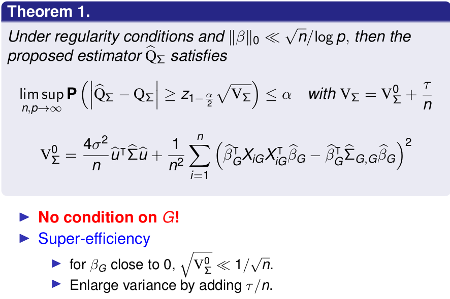
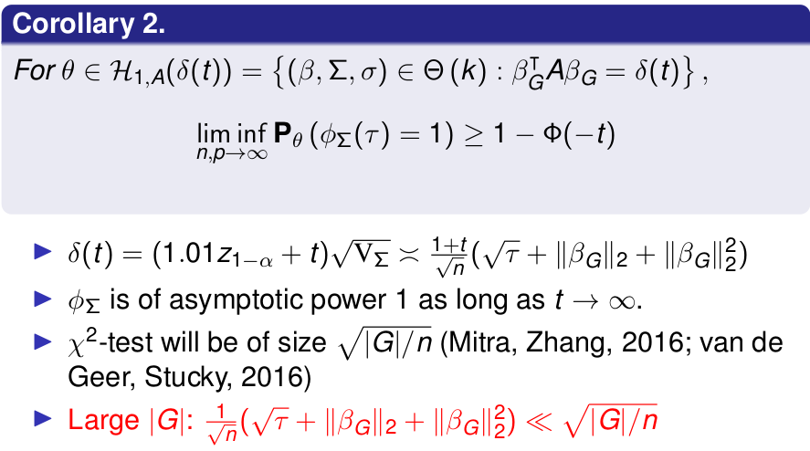
Size and Power
References
- Zhang, C.-H., & Zhang, S. S. (2014). Confidence intervals for low dimensional parameters in high dimensional linear models. Journal of the Royal Statistical Society: Series B (Statistical Methodology), 76(1), 217–242.
- Javanmard, A., & Montanari, A. (2014). Confidence Intervals and Hypothesis Testing for High-Dimensional Regression. 41.