MM algorithm for Variance Components Models

Posted on Nov 01, 2019 (Update: Nov 16, 2023)

Tags: Variance Components Model, Minorization-maximization, Restricted Maximum Likelihood

The post is based on Zhou, H., Hu, L., Zhou, J., & Lange, K. (2019). MM Algorithms for Variance Components Models. Journal of Computational and Graphical Statistics, 28(2), 350–361.

Variance components estimation and mixed model analysis are central themes in statistics with applications in numerous scientific disciplines. MLE and restricted MLE of variance component models remain numerically challenging.

Building on the minorization-maximization (MM) principle, the paper presents a novel iterative algorithm for variance components estimation.

The authors claim that the MM algorithm is trivial to implement and competitive on large data problems, and the algorithm readily extends to more complicated problems such as linear mixed models, multivariate response models possibly with missing data, maximum a posteriori estimation, and penalized estimation.

establish the global convergence of the MM algorithm to a Karush-Kuhn-Tucker point and demonstrate that it converges faster than the classical EM algorithm when the number of variance components is greater than two and all covariance matrices are positive definite.

Introduction

Given an observed $n\times 1$ response vector $y$ and $n\times p$ predictor matrix $X$, the simplest variance components model postulates that $Y\sim N(X\beta, \Omega)$, where $\Omega = \sum_{i=1}^m\sigma_i^2V_i$, and the $V_1,\ldots,V_m$ are $m$ fixed positive semidefinite matrices.

The parameter of the model can be divided into mean effects $\beta = (\beta_1,\ldots,\beta_p)$ and variance components $\sigma^2=(\sigma_1^2,\ldots,\sigma_m^2)$.

Throughout assume $\Omega$ is positive definite.

Estimation resolves around the log-likelihood function

$$L(\beta,\sigma^2) = -\frac 12\log \det\Omega - \frac 12(y-X\beta)^T\Omega^{-1}(y-X\beta)\,.$$

Two popular methods among the commonly used methods for estimating variance components,

• MLE
• restricted (or residual) MLE (REML): first projects $y$ to the null space of $X$ and then estimates variance components based on the projected responses. If the columns of a matrix $B$ span the null space of $X^T$, then REML estimates the $\sigma_i^2$ by maximizing the log-likelihood of the redefined response vector $B^TY$, which is normally distributed with mean 0 and covariance $B^T\Omega B=\sum_{i=1}^m\sigma_i^2B^TV_iB$.

Adopted from Harville, D. A. (1977). Maximum Likelihood Approaches to Variance Component Estimation and to Related Problems. Journal of the American Statistical Association, 72(358), 320–338.

Put $p^* = \rank(\X)$. An error contrast means that a linear combinations $u’y$ of the observations such that $E(u’y)=0$, i.e., such that $u’X=0$. The maximum possible number of linearly independent error contrasts in any set of error contrasts is $n-p^*$. A particular set of $n-p^*$ linearly independent rows of the matrix $\I-\X(\X’\X)^-\X’$. In the REML approach, the inference are based on the likelihood associated with $n - p^*$ linearly independent error contrasts rather than on that associated with the full data vector $y$.

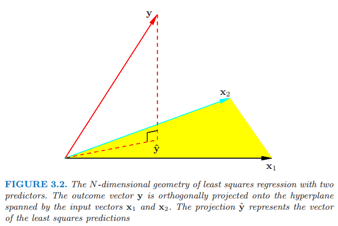
borrow a figure from ESL, the projection $y$ to the null space of $X$ should be the residual vector $y-\hat y$

Estimation bias in variance components originates from the DoF loss in estimating mean components. For the simple linear regression $y=X\beta+\varepsilon, \varepsilon\sim N(0, \sigma^2I)$,

$$\hat\sigma^2_{MLE} = \frac 1N (y-X\hat\beta)^T(y-X\hat\beta)\qquad \text{vs} \qquad \hat\sigma^2_{unbiased} = \frac{1}{N-k}(y-X\hat\beta)^T(y-X\hat\beta)\,,$$

where $k = rank(X(X^TX)^{-1}X^T)$. In such a simple example, we can remove the bias post hoc by multiplying a correction factor. However, for complex problems where closed-form solutions do not exist, we need to resort to ReML.

For general linea regression model, $\varepsilon\sim N(0, H(\theta))$. If vector $a$ is orthogonal to all columns of $X$, i.e., $a^TX=0$, then $a^Ty$ is known as an error contrast. We can find at most $N-k$ such vectors that are linearly independent. Take $A=\begin{bmatrix}a_1 & a_2 &\cdots & a_{N-k}\end{bmatrix}$. It follows that $A^TX=0$ and $E[A^Ty]=0$.

$S = I-X(X^TX)^{-1}X^T$ is a candidate set for $A$. The error contrast vector $w = A^T\varepsilon\sim N(0, A^THA)$ is free of $\beta$. The directly estimate $\theta$ by maximizing a “restricted” log-likelihood function $L(\theta\mid A^Ty)$.

In the simplest linear regression, the mean estimate $\hat\beta$ is independent of the variance component $\theta$. It implies that although the ML and ReML estimates of $\sigma^2$ are different, the estimate of $\hat\beta$ are the same. But it is not true for more complex regression models.

A large literature on iterative algorithms for finding MLE and REML. Fitting variance components models remains a challenge in models with a large sample size $n$ or a large number of variance components $m$.

• Newton’s method converges quickly but is numerically unstable owing to the non-concavity of the log-likelihood
• Fisher’s scoring algorithm replaces the observed information matrix in Newton’s method by the expected information matrix and yields an ascent algorithm when safeguarded by step halving. It is too expensive.
• EM is easy to implement and numerically stable, but painfully slow to converge.

The paper derives a novel minorization-maximization algorithm for finding the MLE and REML estimates of variance components, and prove global convergence of the MM algorithm to a Karush-Kuhn-Tucker (KKT) point and explain why MM generally converges faster than EM for models with more than two variance components.

Preliminaries

Background on MM algorithms

The MM principle for maximizing an objective function $f(\theta)$ involves minorizing the objective function $f(\theta)$ by a surrogate function $g(\theta\mid \theta^{(t)})$ around the current iterate $\theta^{(t)}$ of a search. Minorization is defined by the two conditions

$$\begin{align*} f(\theta^{(t)}) &= g(\theta^{(t)}\mid \theta^{(t)})\\ f(\theta) &\ge g(\theta\mid \theta^{(t)}) \end{align*}$$

The point $\theta^{(t+1)}$ maximizing $g(\theta\mid\theta^{(t)})$ satisfies the ascent property $f(\theta^{(t+1)})\ge f(\theta^{(t)})$.

The celebrated EM principle is a special case of the MM principle. The $Q$ function produced in the E step of an EM algorithm minorizes the log-likelihood up to an irrelevant constant. Thus, both EM and MM share the same advantages: simplicity, stability, graceful adaptation to constraints, and the tendency to avoid large matrix inversion.

Convex Matrix Functions

A matrix-valued function $f$ is said to be matrix convex if

$$f(\lambda A+(1-\lambda)B) \preceq \lambda f(A) + (1-\lambda) f(B)$$

for all $A, B$ and $\lambda\in [0, 1]$.

• the matrix fractional function $f(A, B)=A^TB^{-1}A$ is jointly convex in the $m\times n$ matrix $A$ and the $m\times m$ positive-definite matrix $B$.
• the log determinant function $f(B)=\log\det B$ is concave on the set of positive-definite matrices.

References

• Zhang, Xiuming. “A Tutorial on Restricted Maximum Likelihood Estimation in Linear Regression and Linear Mixed-Effects Model,” 2015