Interior-point Method
Posted on
Nocedal and Wright (2006) and Boyd and Vandenberghe (2004) present slightly different introduction on Interior-point method. More specifically, the former one only considers equality constraints, while the latter incorporates the inequality constraints.
Nocedal and Wright (2006)
Consider the LP problem in standard form,
\[\begin{equation} \min c^Tx,\quad\text{subject to }Ax=b, x\ge 0\,,\label{primal} \end{equation}\]where $c,x\in\IR^n$ and $b\in\IR^m$, and $A$ is an $m\times n$ matrix with full row rank.
The dual problem is
\[\begin{equation} \max b^T\lambda,\quad \text{subject to }A^T\lambda+s=c,s\ge 0\,,\label{dual} \end{equation}\]where $\lambda\in \IR^m$ and $s\in \IR^n$. Solutions of \eqref{primal} and \eqref{dual} can be characterized by the KKT conditions,
\[\begin{align*} A^T\lambda + s&=c\\ Ax&=b\\ x_is_i&=0,i=1,2,\ldots,n,\\ (x,s)&\ge 0\,. \end{align*}\]Restate the optimality conditions in a slightly different form by means of a mapping $F$ from $\IR^{2n+m}$ to $\IR^{2n+m}$:
\[\begin{align*} F(x,\lambda, s) = \begin{bmatrix} A^T\lambda +s -c \\ Ax-b\\ XSe\\ \end{bmatrix} &=0\\ (x,s)&\ge 0 \end{align*}\,,\]where $X=\diag(x_1,\ldots,x_n), S=\diag(s_1,\ldots,s_n)$ and $e=(1,\ldots,1)^T$. Primal-dual methods generates iterates $(x^k,\lambda^k,s^k)$ that satisfy the bounds strictly, i.e., $x^k > 0$ and $s^k > 0$. This property is the origin of the term interior-point.
Like most iterative algorithms in optimization, primal-dual interior-point methods have two basic ingredients: a procedure for determining the step and a measure of the desirability of each point in the search space.
Firstly, the duality measure is defined by
\[\mu = \frac 1n\sum_{i=1}^n x_is_i = \frac{x^Ts}{n}\,.\]The procedure for determining the search direction has its origins in Newton’s method. Newton’s method forms a linear model for F around the current point and obtains the search direction $(\Delta x,\Delta \lambda, \Delta s)$ by solving the following system of linear equations
\[J(x,\lambda, s)\begin{bmatrix} \Delta x\\ \Delta \lambda \\ \Delta s \end{bmatrix} = -F(x,\lambda, s)\,,\]where $J$ is the Jacobian of $F$. Let $r_c$ and $r_b$ be the first two block rows in $F$,
\[r_b=Ax-b,\qquad r_c=A^\lambda+s-c\,,\]then
\[\begin{bmatrix} 0 & A^T & I\\ A & 0 & 0\\ S & 0 & X \end{bmatrix} \begin{bmatrix} \Delta x\\ \Delta \lambda\\ \Delta s \end{bmatrix}= \begin{bmatrix} -r_c\\ -r_b\\ -XSe \end{bmatrix}\,.\]Note that $J_{ij} = \frac{\partial f_i}{\partial x_j}$, i.e., $J_{i\cdot} = \frac{\partial f_i}{\partial x’}$, so we have $\frac{\partial f_1}{\partial \lambda’} = A^T$.
Usually a full step along this direction would violate the bound $(x,s)\ge 0$, so we perform a line search along the Newton direction and define the new iterate as
\[(x,\lambda, s) + \alpha (\Delta x,\Delta \lambda, \Delta s)\,,\]for some line search parameter $\alpha\in (0,1]$. We often can take only a small step along this direction ($\alpha < < 1$) before violating the condition $(x,s) > 0$. Hence, the pure Newton direction, sometimes known as the affine scaling direction, often does not allow us to make much progress toward a solution.
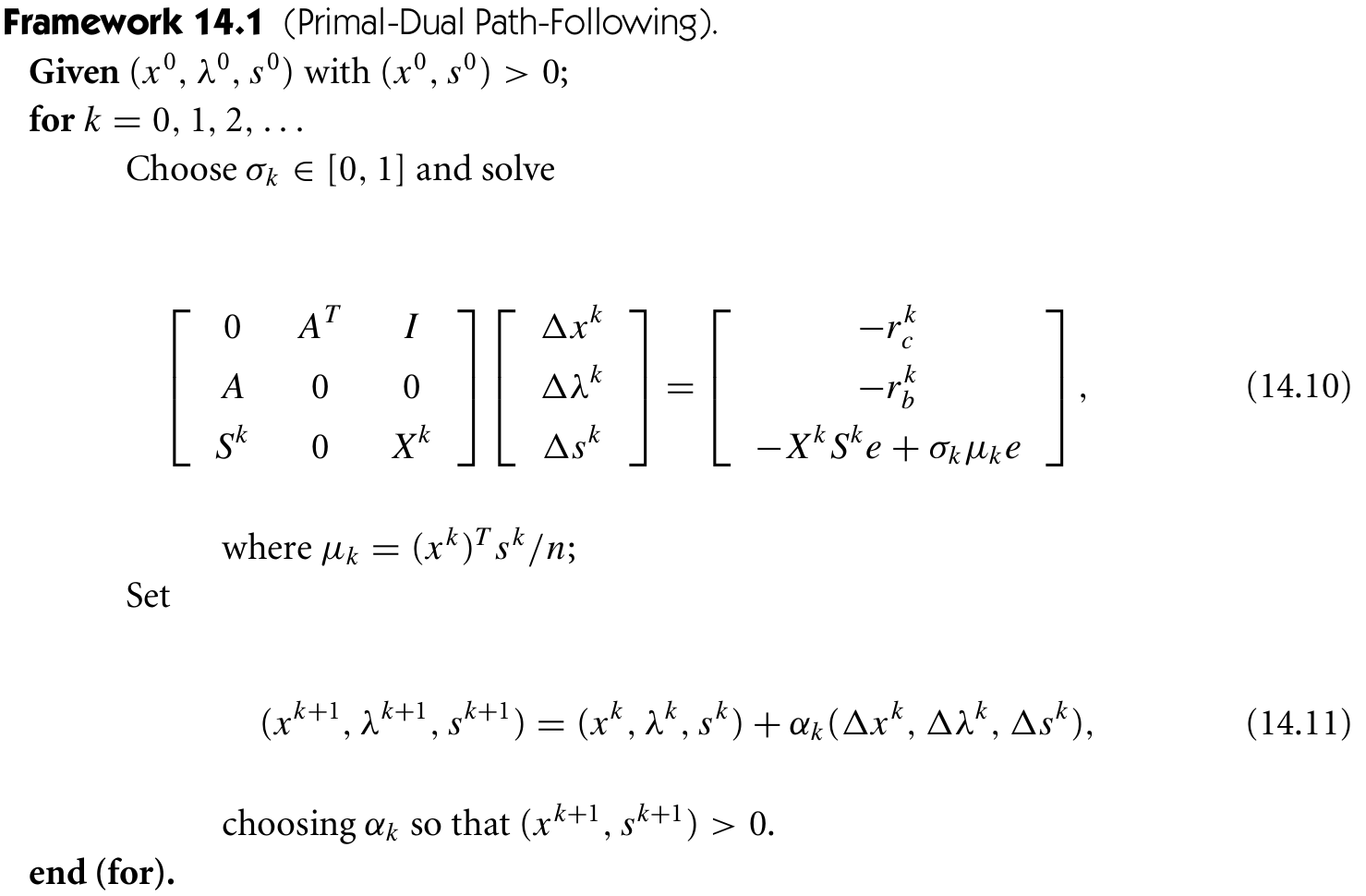
Most primal-dual methods use a less aggressive Newton direction, aim for a point whose pairwise products $x_is_i$ are reduced to a lower average value–not all the way to zero. Take a Newton step toward the point for which $x_is_i=\sigma\mu$, where $\mu$ is the current duality measure and $\sigma\in[0, 1]$ is the reduction factor that we wish to achieve in the duality measure on this step. The modified step equation is then
\[\begin{bmatrix} 0 & A^T & I\\ A & 0 & 0\\ S & 0 & X \end{bmatrix} \begin{bmatrix} \Delta x\\ \Delta \lambda\\ \Delta s \end{bmatrix}= \begin{bmatrix} -r_c\\ -r_b\\ -XSe+\sigma\mu e \end{bmatrix}\,.\]Here $\sigma$ is called the centering parameter.
Actually, software for implementing interior-point methods does not usually start from a feasible point $(x^0,\lambda^0,s^0)$.
Central Path
- feasible set $\cF=\{(x,\lambda,s)\mid Ax=b,A^T\lambda+s=c,(x,s)\ge 0\}$
- strictly feasible set $\cF^0 = \{(x,\lambda,s)\mid Ax=b,A^T\lambda+s=c,(x,s)> 0\}$
The central path $\cC$ is an arc of strictly feasible points, which is parametrized by a scalar $\tau > 0$, and each point $(x_\tau,\lambda_\tau,s_\tau)\in\cC$ satisfies the following equations:
\[\begin{align*} A^T\lambda + s &= c\\ Ax &= b\\ x_is_i &=\tau,\qquad i=1,2,\ldots,n\\ (x,s) &> 0 \end{align*}\]Then define the central path as
\[\cC = \{(x_\tau,\lambda_\tau,s_\tau)\mid \tau > 0\}\,.\]Central Path Neighborhoods and Path-Following Methods
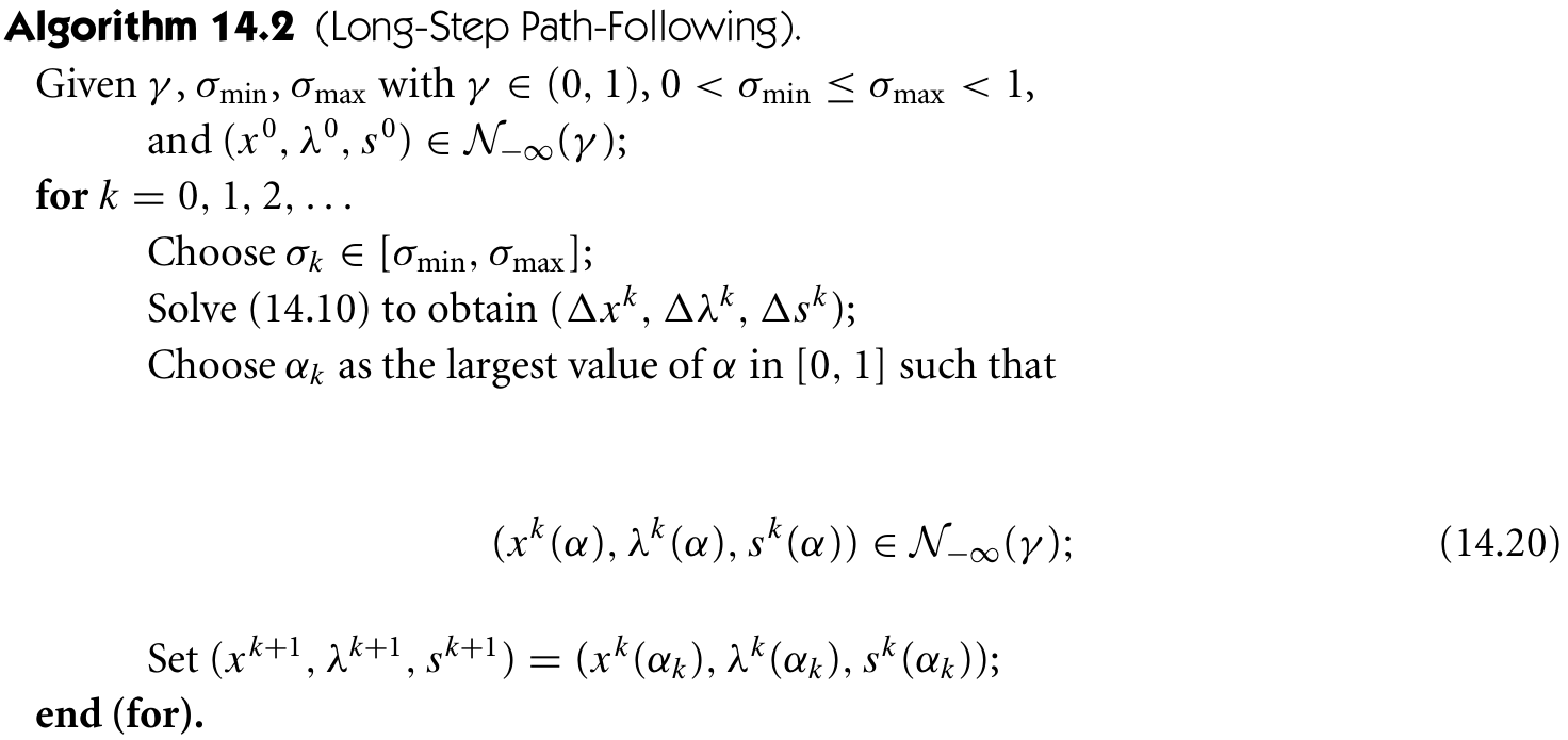
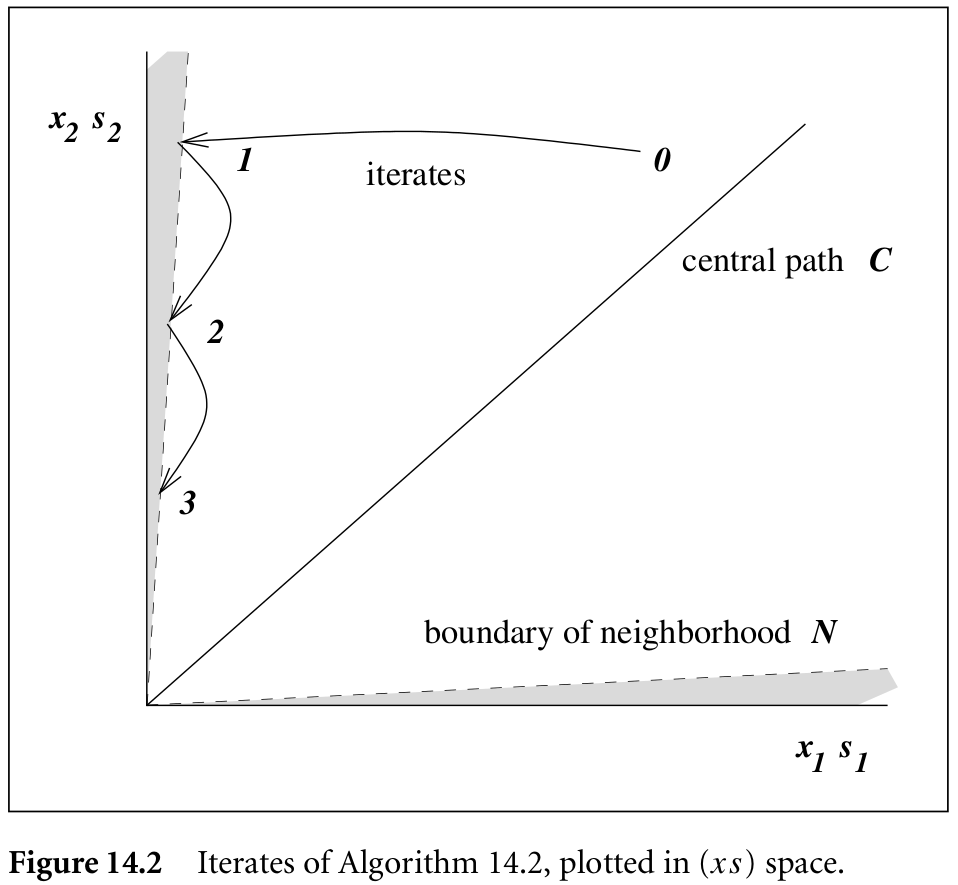
Path-following algorithms explicitly restrict the iterates to a neighborhood of the central path $\cC$ and follow $\cC$ to a solution of the linear program.
Two most interesting neighborhood of $\cC$ are
- $\cN_2(\theta) = \{(x,\lambda, s)\in \cF^o\mid \Vert XSe-\mu e\Vert_2\le \theta\mu\}$ for some $\theta\in [0,1)$
- $\cN_{-\infty}(\gamma) = \{(x,\lambda, s)\in \cF^o\mid x_is_i\ge \gamma\mu\;\forall i=1,2\ldots,n\}$
Boyd and Vandenberghe (2004)
Consider the convex optimization problems that include inequality constraints,
\[\begin{equation} \min f_0(x)\quad \text{subject to }f_i(x)\le 0,i=1,\ldots,m\,, Ax=b\,,\label{11.1} \end{equation}\]where $f_0,\ldots,f_m:\IR^n\rightarrow \IR$ are convex and twice continuously differentiable, and $A\in \IR^{p\times n}$ with rank $p < n$.
- Assume that the problem is solvable, i.e., an optimal $x^\star$ exists. Denote the optimal value $f_0(x^\star)$ as $p^\star$.
- Assume that the problem is strictly feasible, i.e., there exists $x\in\cD$ that satisfies $Ax=b$ and $f_i(x) < 0$ for $i=1,\ldots,m$.
Thus, there exist dual optimal $\lambda^\star\in\IR^m,\nu^\star\in\IR^p$, which together with $x^\star$ satisfy the KKT conditions
\[\begin{align*} Ax^\star =b, f_i(x^\star) &\le 0,i=1,\ldots,m\\ \lambda^\star &\succeq 0\\ \nabla f_0(x^\star) + \sum_{i=1}^m \lambda_i^\star \nabla f_i(x^\star) + A^T\nu^\star &=0\\ \lambda_i^\star f_i(x^\star) &= 0,i=1,\ldots,m\,. \end{align*}\]Logarithmic barrier function and central path
The goal is to approximately formulate the inequality constrained problem as an equality constrained problem to which Newton’s method can be applied.
Rewrite \eqref{11.1} to make the inequality constraints implicit in the objective,
\[\min f_0(x) + \sum_{i=1}^mI_{\_}(f_i(x))\quad\text{subject to }Ax=b\,,\]where $I_{\_}:\IR\rightarrow \IR$ is the indicator function for the nonpositive reals,
\[I_{\_}(u) = \begin{cases} 0 & u\le 0\\ \infty & u > 0 \end{cases}\,.\]The basic idea of the barrier method is to approximate the indicator function $I_{\_}$ by the function
\[\hat I_{\_}(u) = -(1/t)\log(-u)\,, \text{dom} \hat I_{\_} = -\IR_{++}\,,\]where $t>0$ is a parameter that sets the accuracy of the approximation. Unlike $I_{\_ }$, $\hat I_{\_}$ is differentiable and closed: it increases to $\infty$ as $u$ increases to 0.
Thus, we have the approximation
\[\min f_0(x)+\sum_{i=1}^m -(1/t)\log(-f_i(x))\quad \text{subject to }Ax=b\,.\]The function
\[\phi(x) = -\sum_{i=1}^m\log (-f_i(x))\]with $\text{dom} \phi=\{x\in\IR^n\mid f_i(x) < 0,i=1,\ldots,m\}$ is called the logarithmic barrier or log barrier.
We can simplify notation if multiplying the objective by $t$, and get the equivalent problem
\[\begin{equation} \min tf_0(x) + \phi(x)\quad\text{subject to }Ax=b\,.\label{11.6} \end{equation}\]For $t > 0$, define $x^\star(t)$ as the solution of \eqref{11.6}. The central path associated with problem \eqref{11.1} is defined as the set of points $x^\star(t), t>0$, which we call the central points. Points on the central path are characterized by the following necessary and sufficient conditions: $x^\star(t)$ is strictly feasible, i.e., satisfies
\[Ax^\star(t) = b,\quad f_i(x^\star(t)) < 0,\quad i=1,\ldots,m\,,\]and there exists a $\hat \nu\in\IR^p$ such that
\[\begin{align} 0 &= t\nabla f_0(x^\star(t)) + \nabla \phi(x^\star(t)) + A^T\hat\nu\\ &=t\nabla f_0(x^\star(t)) + \sum_{i=1}^m\frac{1}{-f_i(x^\star(t))}\nabla f_i(x^\star(t)) + A^T\hat\nu\label{11.7}\,. \end{align}\]It follows that every central point yields a dual feasible point, and hence a lower bound on the optimal value $p^\star$. More specifically, define
\[\lambda_i^\star(t) = -\frac{1}{tf_i(x^\star(t))},\quad i=1,\ldots,m,\quad \nu^\star(t)=\hat\nu /t\,.\]It claims that the pair $\lambda^\star(t),\nu^\star(t)$ is dual feasible.
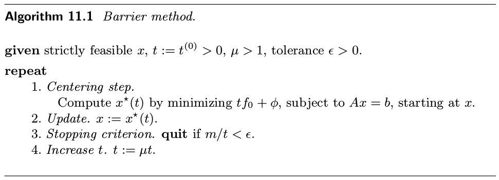
The barrier method
Take $t=m/\epsilon$,
The central path conditions \eqref{11.7} can be interpreted as a continuous deformation of the KKT optimality conditions. A point $x$ is equal to $x^\star(t)$ iff there exists $\lambda,\mu$ such that
\[\begin{align*} Ax = b, f_i(x) &\le 0,i=1,\ldots,m\\ \lambda &\succeq 0\\ \nabla f_0(x) + \sum_{i=1}^m\lambda_i\nabla f_i(x) + A^T\nu &= 0\\ -\lambda_if_i(x) &=1/t,i=1,\ldots,m\,, \end{align*}\]which can be solved by Newton step (ignoring the inequality).
Firstly, we can eliminate the variables $\lambda_i = -1/(tf_i(x))$,
\[\begin{align*} \nabla f_0(x) + \sum_{i=1}^m\frac{1}{-tf_i(x)}\nabla f_i(x) + A^T\nu &= 0\\ Ax &=b\,. \end{align*}\]Write in matrix form,
\[G(x,\nu) = \begin{bmatrix} t\nabla f_0(x) + \nabla \phi(x) + tA^T\nu \\ Ax-b \end{bmatrix}=0\,,\]then we can get the Newton step.
Primal-dual search direction
Define
\[r_t(x,\lambda,\nu) = \begin{bmatrix} \nabla f_0(x) + Df(x)^T\lambda + A^T\nu\\ -\diag(\lambda)f(x) -(1/t)\1\\ Ax-b \end{bmatrix}\]and $t > 0$. The first block component of $r_t$,
\[r_{dual} = \nabla f_0(x) + Df(x)^T\lambda + A^T\nu\,,\]is called the dual residual, and the last block component, $r_{pri}=Ax-b$ is called the primal residual. The middle block,
\[r_{cent} = -\diag(\lambda)f(x) - (1/t)\1\,,\]is the centrality residual. The Newton step is
\[\begin{bmatrix} \nabla^2f_0(x) + \sum_{i=1}^m\lambda_i\nabla^2f_i(x) & Df(x)^T & A^T\\ -\diag(\lambda)Df(x) & -\diag(f(x)) & 0 \\ A & 0 & 0 \end{bmatrix} \begin{bmatrix} \Delta x\\ \Delta \lambda\\ \Delta \nu \end{bmatrix} = -\begin{bmatrix} r_{dual}\\ r_{cent}\\ r_{pri} \end{bmatrix}\,.\]