Surprises in High-Dimensional Ridgeless Least Squares Interpolation

Posted on Jun 24, 2019 (Update: Nov 30, 2021)

Tags: Interpolation, High-Dimensional, Deep Neural Networks, Risk Function, Cross-Validation, Probability Measure, Random Matrix Theory

This post is based on Hastie, T., Montanari, A., Rosset, S., & Tibshirani, R. J. (2019). Surprises in High-Dimensional Ridgeless Least Squares Interpolation. 53.

Introduction

• Zhang et al. (2016) showed that state-of-art deep neural network architectures are complex enough that they can be trained to interpolate the data even when the actual labels are replaced by entirely random ones in a thought-provoking experiment.
• Deep neural networks are frequently observed to generalize well in practice despite their enormous complexity. It seems to defy conventional statistical wisdom: interpolation (vanishing training error) is commonly taken to be a proxy for overfitting or poor generalization.
  • Belkin et al. (2018bca) pointed out that these concepts are in general distinct, and interpolation does not contradict generalization.
  • Estimation in RKHS is a well-understood setting in which interpolation can coexist with good generalization (Liang and Rakhlin, 2018)

What least squares has to do with neural networks

Suppose that we have a nonlinear model $\bbE(y_i\mid z_i)=f(z_i;\theta)$ relating responses $y_i\in\bbR$ to inputs $z_i\in\bbR^d,i=1,\ldots,n$, via a parameter vector $\theta\in\bbR^p$.

In some problems, the number of parameters $p$ is so large that training effectively moves each of them just a small amount w.r.t. some random initialization $\theta_0\in\bbR^p$. It thus makes sense to linearize the model around $\theta_0$.

Further, supposing that the initialization is such that $f(z;\theta_0)\approx 0$, and letting $\theta = \theta_0+\beta$, then

\[\bbE(y_i\mid z_i) \approx \nabla_\theta f(z_i;\theta_0)^T\beta,\qquad i=1,\ldots,n.\]

Therefore, we are led to consider a linear regression problem, with random features $x_i=\nabla_\theta f(z_i;\theta_0),i=1,\ldots,n$ of high-dimensionality ($p$ much greater than $n$).

In this setting, many vectors $\beta$ give rise to a model that interpolates the data. However, using gradient descent on the least squares objective for training yields a special interpolating parameter $\hat\beta$ (having implicit regularity): the least squares solution with minimum $\ell_2$ norm.

Two different models for the feature distribution.

• a linear model, $x_i=\Sigma^{1/2}z_i\in \bbR^p$, where $z_i\in\bbR^p$ has iid entries with zero mean and unit variance and $\Sigma\in\bbR^{p\times p}$ deterministic and positive definite. This is a standard model in random matrix theory, and we can obatin a fairly complete asymptotic characterization of the out-of-sample prediction risk.
• a nonlinear model, $x_i=\phi(Wz_i)\in\bbR^p$ with $z_i\in\bbR^d, W\in \bbR^{p\times d}$, and $\phi$ an activation function acting componentwise on $Wz_i$.

The authors recover, in a precise quantitative way, several phenomena that have been observed in large-scale neural networks and kernel machine, including “double descent” behaviour of the prediction risk, and the potential benefits of overparametrization.

Summary of results

Analyze the out-of-sample prediction risk of the minimum $\ell_2$ norm (min-norm, for short) least squares estimator, in an asymptotic setup where both the number of samples and features diverge, $n,p\rightarrow \infty$, and their ratio convergences to a nonzero constant, $p/n\rightarrow \gamma\in (0,\infty)$.

• $\gamma < 1$: underparametrized
• $\gamma > 1$: overparametrized

The results are:

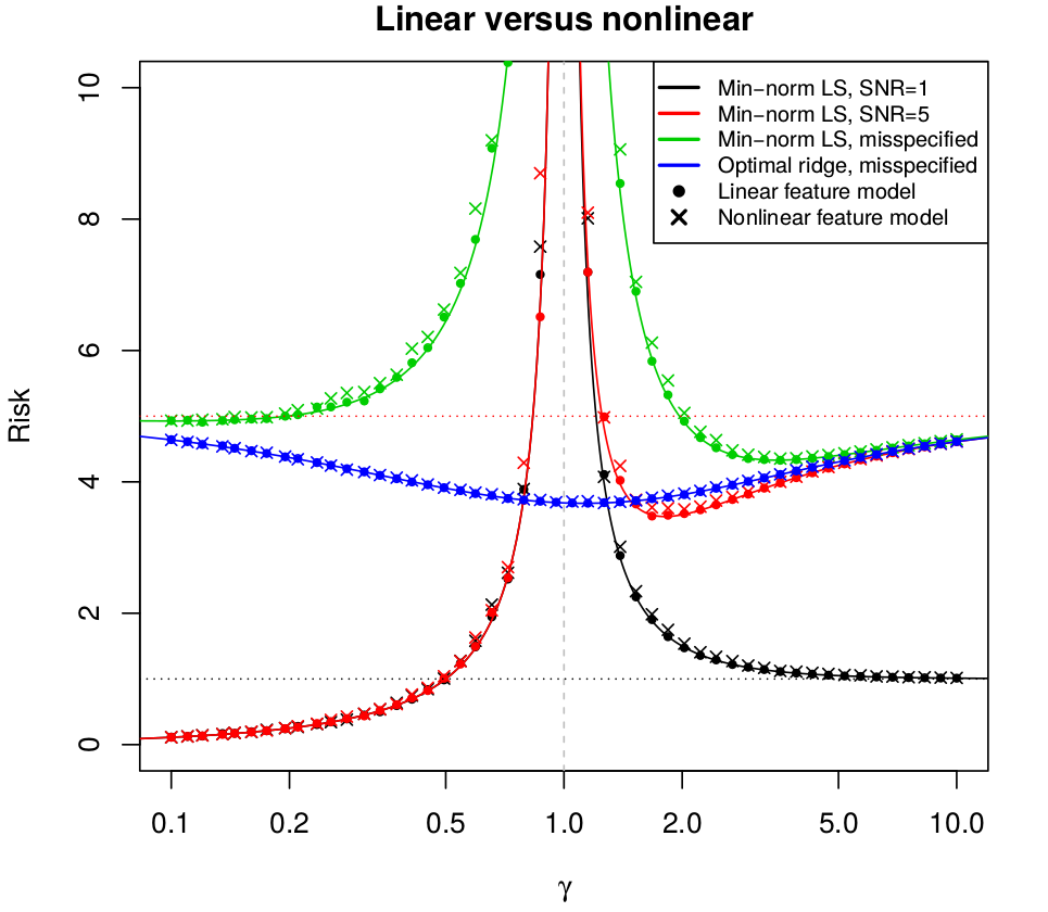
0. If $\gamma < 1$, the risk is purely variance (there is no bias), and does not depend on $\beta,\Sigma$. Moreover, the risk diverges as we approach the interpolation boundary (as $\gamma\rightarrow 1$)a known result that has appeared in various places in the random matrix theory literature
1. If $\gamma > 1$, the risk is composed of both bias and variance, and generally depends on $\beta,\Sigma$. In the two models, the bias is decreasing with strength of correlation, and the variance is nondecreasing.
2. If $\SNR \le 1$, the risk is decreasing for $\gamma\in (1,\infty)$, and approaches the null risk (from above) as $\gamma \rightarrow\infty$
3. If $\SNR > 1$, the risk has a local minimum on $\gamma\in (1,\infty)$, is better than the null risk for large enough $\gamma$, and approaches the null risk (from below) as $\gamma \rightarrow \infty$.
4. For a misspecified model, when $\SNR >1$, the risk can attain its global minimum on $\gamma\in(1,\infty)$ (when there is strong enough approximation bias)
5. Optimally-tuned ridge regression dominates the min-norm least squares estimator in risk, across all values of $\gamma$ and SNR, in both the well-specified and misspecified settings. For a misspecified model, optimally-tuned ridge regression attains its global minimum around $\gamma=1$
6. Tuning ridge regression by minimizing the leave-one-out cross-validation (CV) error is asymptotically optimalpoints 3 through 6 are formally established for isotropic features, $\Sigma=I$, but qualitatively similar behavior holds for general $\Sigma$.
7. For the nonlinear model, as $n,p,d\rightarrow \infty$, with $p/n\rightarrow\gamma\in(0,\infty)$ and $d/p\rightarrow\psi\in(0,1)$, the limiting variance is increasing for $\gamma\in (0,1)$, decreasing for $\gamma\in(1,\infty)$, and diverging as $\gamma\rightarrow 1$. In fact, if $\gamma < 1$, the variance coincides exactly with one in the linear model case
8. If $\gamma > 1$, the asymptotic formula for the variance in the nonlinear model depends only on the activation function $\psi$ via its “linear component” $\bbE[G\phi(G)]$.
9. If $\gamma > 1$, for a “purely nonlinear” activation function $\psi$, meaning $\bbE[G\psi(G)]=0$, the asymptotic formula for the variance coincides with the one derived for the linear model case, despite the fact that the input dimension $d$ can be much smaller than the number of parameters $p$.the nonlinear model results are not covered by existing literature on random matrix theory

Intuition and Implications

Bias and Variance

When $p > n$, the min-norm least squares estimate of $\beta$ is constrained to lie the row space of $X$. This is a subspace of dimension $n$ lying in a feature space of dimension $p$.

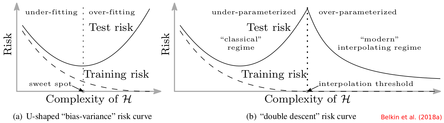
Double Descent

Belkin et al. (2018a)

In-sample prediction risk

The focus throughout this paper is out-of-sample prediction risk.

For the two models, the in-sample prediction risk of the min-norm least squares estimator $\hat\beta$ is

\[\frac 1n\bbE[\Vert X\hat\beta - X\beta\Vert_2^2\mid X] = \sigma^2(p/n \land 1)\,.\]

\[\begin{align*} \bbE[\Vert X\hat\beta - X\beta\Vert_2^2\mid X] &= \bbE[(\hat\beta-\beta)'X'X(\hat\beta-\beta)\mid X]\\ &=\tr[X'X\Cov(\hat\beta)] + (E(\hat\beta)-\beta)'X'X(E(\hat\beta) - \beta)\\ \end{align*}\]

where $E(\hat\beta) = \beta$, and $\Cov(\hat\beta)=(X’X)^+\sigma^2$. If $p > n$,

\[X'X = V \begin{bmatrix} \Lambda_n & \\ & 0_{p-n} \end{bmatrix} V'\]

then

\[(X'X)^+ = V \begin{bmatrix} \Lambda_n^{-1} & \\ & 0_{p-n} \end{bmatrix} V'\,.\]

The following simple Julia snippet can be used to validate the above relationship.

X = randn(10, 20)
A = X' * X
Λ, V = eigen(A)
Λ1 = Λ[11:end]
Λ2 = vcat(zeros(10), 1 ./ Λ1)
norm(V * diagm(Λ2) * V' - pinv(A), 2)
# 3.027733893412882e-15

The in-sample prediction risk is not always a good proxy for the out-of-sample prediction risk. Although much of classical regression theory is based on the former, such as optimism, effective degrees of freedom, and covariance penalities, the latter is more broadly relevant to practice.

Interpolation versus Regularization

It is worthy noting that early stopped gradient descent is known to be closely connected to ridge regularization.

A tight coupling between the two has been recently developed for least squares problems. This coupling implies that optimally-stopped gradient descent will have risk at most 1.22 times that of optimally-tuned ridge regression, and hence will often have better risk than min-norm least squares.

In practice, we would not have access to the optimal tuning parameter for ridge, and would rely on CV. The theory shows that for ridge regression, CV tuning is asymptotically equivalent to optimal tuning.

Historically, the debate between interpolation and regularization has been alive for the last 30 or so years.

Virtues of nonlinearity

It is unclear whether the success in precisely analyzing the linear model setting should carry over to the nonlinear setting. Remarkably, under high-dimensional asymptotics with $n,p,d\rightarrow\infty,p/n\rightarrow \gamma$, and $d/p\rightarrow\psi$, this turns out to be the case.

There is a critical difference between neural networks and the studies in this paper: in a neural network, the feature representation and the regression function or classifier are learned simultaneously. In both linear and nonlinear model settings, the features $X$ are not learned, but observed.

Preliminaries

Data model and risk

• training data: $(x_i, y_i)\in \IR^p \times \IR,i=1,\ldots,n$
• test point: $x_0\sim P_x$

For an estimator $\hat\beta$ (a function of the training data $X, y$), define its out-of-sample prediction risk

\[R_X(\hat\beta,\beta) = \E[(x_0^T\hat\beta - x_0^T\beta)^2\mid X]=\E[\Vert \hat\beta - \beta\Vert_\Sigma^2\mid X]\,,\]

where $\Vert x\Vert_\Sigma^2 = x^T\Sigma x$.

It has the bias-variance decomposition

\[R_X(\hat\beta;\beta) = \Vert \E(\hat\beta\mid X) - \beta\Vert_\Sigma^2 + \tr[\Cov(\hat\beta\mid X)\Sigma] = B_X(\hat\beta;\beta) + V_X(\hat\beta;\beta)\]

Generally, the risk function measures the accuracy of an estimator $\delta(\theta)$ for parameter $\theta$, $R(\theta,\delta) = E_\theta[L(\theta, \delta(X))]$. Two natural global measures of the size of the risk are the average $\int R(\theta, \delta)w(\theta)d\theta$ (Bayes) and the maximum $\sup_\Omega R(\theta,\delta)$ (minimax).

Theorem 7 and Its Proof

Assume an isotropic prior, namely $E(\beta)=0,Cov(\beta)=r^2I_p/p$, and data model

\[\begin{align*} (x_i,\epsilon_i) & \sim P_x\times P_\epsilon, i=1,\ldots,n\\ y_i &= x_i^T\beta + \epsilon_i, i=1,\ldots,n\,, \end{align*}\]

Assume that $x\sim P_x$ has i.i.d. entries with zero mean, unit variance, and a finite moment of order $4+\eta$, for some $\eta > 0$. Then for the CV error

\[CV_n(\lambda) = \frac 1n\sum_{i=1}^n(y_i-\hat f_\lambda^{-i}(x_i))^2\]

of the ridge estimator in

\[\hat\beta_\lambda = \arg\min_{b\in\IR^p}\left\{\frac 1n \Vert y-Xb\Vert_2^2 + \lambda \Vert b\Vert^2_2\right\}\]

with tuning parameter $\lambda > 0$, as $n, p\rightarrow \infty$, with $p/n\rightarrow \gamma\in (0,\infty)$ , it holds almost surely that

\[CV_n(\lambda) - \sigma^2 \rightarrow \sigma^2\gamma(m(-\lambda)-\lambda(1-\alpha\lambda)m'(-\lambda))\,,\]

where $m(z)$ denotes the Stieltjes transform of the Marchenko-Pastur law $F_\gamma$, and $\alpha = r^2/(\sigma^2\gamma)$. Observe that the right-hand side is the asymptotic risk of ridge regression from Theorem 6. Moreover, the above convergence is uniform over compacts intervals excluding zero. Thus if $\lambda_1,\lambda_2$ are constants with $0 < \lambda_1\le \lambda^\star \le \lambda_2 < \infty$, where $\lambda^\star = 1/\alpha$ is the asymptotically optimal ridge tuning parameter value, and we define $\lambda_n=\arg\min_{\lambda\in[\lambda_1,\lambda_2]}CV_n(\lambda)$, then the risk of the CV-tuned ridge estimator $\hat\beta_{\lambda_n}$ satisfies, almost surely,

\[R_X(\hat\beta_{\lambda_n}) \rightarrow \sigma^2\gamma m(-1/\alpha)\,,\]

with the right-hand side above being the asymptotic risk of optimally-tuned ridge regression. Further, the exact same set of results holds for GCV.

The asymptotic results are similar in spirit to old results, but the details differ: owing to the random matrix theory approach, one can establish the (stronger) result that the CV and GCV error curves converge uniformly to the ridge prediction error curve, by leveraging the fact that they are composed of functionals that have almost sure limits under Marchenko-Pastur asymptotics.

The key implication, in the context of the current paper and its central focus, is that the CV-tuned or GCV-tuned ridge estimator has the same asymptotic performance as the optimally-tuned ridge estimator, and therefore enjoys the same performance gap over min-norm least squares.

Analysis of GCV

Rewrite the GCV criterion

\[GCV_n(\lambda) = \frac{y'(I-S_\lambda)^2y/n}{(1-\tr(S_\lambda)/n)^2}\]

GCV denominator

\[\tr(S_\lambda) / n = \frac 1n \sum_{i=1}^p\frac{s_i}{s_i+\lambda} \rightarrow \gamma\int \frac{s}{s+\lambda}dF_\gamma(s) = \gamma(1-\color{red}{\lambda}m(-\lambda))\]

where the convergence holds almost surely as $n,p\rightarrow \infty$, and $m$ denotes the Stieltjes transform of the MP law $F_\gamma$.

For a counting measure and any Borel function $f$, we have $\int f=\sum_{w\in \Omega} f(w)$ (Example 1.5 of Shao,2003). Now for a discrete CDF, which can be viewed as multiplying $1/n$ on the counting measure, then

\[\int fdF_n(x) = \frac 1n \sum f(x)\,,\]

that is

\[\frac 1p\sum_{i=1}^p\frac{s_i}{s_i+\lambda} = \int \frac{s}{s+\lambda} dF_p(s)\,,\]

where $F_p(x)$ is the empirical spectral distribution (ESD). MP law said that

\[F_p(x)\rightarrow F_\gamma(x)\,, a.s.\]

The Stieltjes transform (wiki) is defined as

\[m(z) = \int \frac{dF(x)}{x-z}\]

so

\[\int \frac{s}{s+\lambda} dF(s) = \int 1-\frac{\lambda}{s+\lambda}dF(s) = 1-\lambda m(-\lambda)\]

which is different from the context.

GCV numerator

Let $y=X\beta + \epsilon$ and $c_n = \sqrt p(\sigma/r)$,

\[y'(I-S_\lambda)^2y/n = (\beta,\varepsilon)^T\left(\frac 1n \begin{bmatrix} X\\ I \end{bmatrix}^T (I-S_\lambda)^2 \begin{bmatrix} X\\ I \end{bmatrix} \right) (\beta,\varepsilon) = (\beta,\varepsilon/c_n)^T\left(\frac 1n \begin{bmatrix} X\\ c_nI \end{bmatrix}^T (I-S_\lambda)^2 \begin{bmatrix} X\\ c_nI \end{bmatrix} \right) (\beta,\varepsilon/c_n)\triangleq \delta'A\delta\]

Note that $\delta$ has independent entries with mean zero and variance $r^2/p$, and further, $\delta$ and $A$ are independent.

Use the almost sure convergence of quadratic forms, we have almost surely

\[\delta'A\delta - r^2/p\tr(A) \rightarrow 0\]

Now examine

\[r^2\tr(A) / p = \frac{r^2}{p}\tr((I-S_\lambda)^2(XX^T/n + c_n^2/nI)) = \frac{r^2}{p}\tr(X'(I-S_\lambda)^2X/n) + \frac{\sigma^2}{n}\tr((I-S_\lambda)^2)\triangleq a+b\]

where

\[a = \frac{r^2\lambda^2}{p}\left(\sum_{i=1}^p\frac{1}{s_i+\lambda} - \lambda\sum_{i=1}^p\frac{1}{(s_i+\lambda)^2}\right)\rightarrow r^2\lambda^2(m(-\lambda)-\lambda m'(-\lambda))\]

and

\[b = \frac{\sigma^2}{n}\left(\sum_{i=1}^p\frac{\lambda^2}{(s_i+\lambda)^2}+(n-p)\right)\rightarrow \sigma^2\gamma\lambda^2m'(-\lambda) + \sigma^2(1-\gamma)\]

Putting together, we have almost surely

\[GCV_n(\lambda) \rightarrow \frac{\lambda^2(r^2(m(-\lambda)-\lambda m'(-\lambda)) + \sigma^2\gamma m'(-\lambda))+\sigma^2(1-\gamma)}{(1-\gamma(1-m(-\lambda)))^2}\]

Reparametrize the above asymptotic limit in terms of the companion Stieltjes transform $v$. This satisfies

\[v(z) + 1/z = \gamma(m(z) + 1/z)\,,\]

hence

\[zv(-z) - 1 = \gamma(zm(-z) - 1)\,,\]

and also

\[z^2v'(-z) - 1 = \gamma(z^2m'(-z) - 1)\,.\]

Introducing $\alpha = r^2/\sigma^2\gamma$, the almost sure limit of GCV is

\[\frac{\sigma^2(v(-\lambda) + (\alpha\lambda-1)(v(-\lambda) - \lambda v'(-\lambda)))}{\lambda v(-\lambda)^2}\]

Recognize the above as $\sigma^2$ plus the asymptotic risk of ridge regression at tuning parameter $\lambda$.

Uniform Convergence

Denote $f_n(\lambda) = GCV_n(\lambda)$, and $f(\lambda)$ for its almost sure limit.

Notice that $\vert f_n\vert$ is almost surely bounded on $[\lambda_1,\lambda_2]$, for large enough $n$, as

\[\begin{align} \vert f_n(\lambda)\vert & \le \frac{\Vert y\Vert^2_2}{n}\frac{\lambda_\max(I-S_\lambda)^2}{(1-\tr(S_\lambda)/n)^2}\\ &\le \frac{\Vert y\Vert_2^2}{n}\frac{(s_\max+\lambda)^2}{\lambda^2}\\ &\le 2(r^2+\sigma^2)\frac{(2+\lambda_2)^2}{\lambda_1^2} \end{align}\]

where $\Vert y\Vert_2^2/n \le 2(r^2+\sigma^2)$ a.s. for sufficiently large $n$, by the strong law of large numbers, and $s_\max \le 2$ a.s. for sufficiently large $n$, by Bai-Yin theorem.

Furthermore, writting $g_n, h_n$ for the numerator and denominator of $f_n$,

• $\vert g_n(\lambda)\vert$ is upper bounded on $[\lambda_1,\lambda_2]$
• $\vert h_n(\lambda)\vert$ is lower bounded on $[\lambda_1,\lambda_2]$ and clearly $\vert h_n(\lambda)\vert\le 1$

To show that $\vert f_n’\vert$ is almost surely bounded on $[\lambda_1,\lambda_2]$, it suffices to show that both $\vert g_n’\vert, \vert h_n’\vert$ are.

Denote by $u_i,i=1,\ldots,p$ the eigenvectors of $X^TX/n$, then

\[\vert g_n'(\lambda)\vert = \frac{2\lambda}{n}\sum_{i=1}^p(u_i^Ty)^2\frac{s_i}{(s_i+\lambda)^3}\le \frac{2\lambda}{n}\Vert y\Vert_2^2 \le 4\lambda(r^2+\sigma^2)\,,\]

the last step holding almost surely for large enough $n$ by the law of large numbers. Also,

\[\vert h_n'(\lambda)\vert = 2\left(1-\frac 1n\sum_{i=1}^n\frac{s_i}{s_i+\lambda}\right)\frac 1n\sum_{i=1}^n\frac{s_i}{(s_i+\lambda)^2}\color{orange}{\le 2\frac{1}{s_1+\lambda}\frac{s_\max}{s_\max + \lambda}}\le \frac{4}{\lambda_1^2}\]

Thus $\vert f_n’\vert$ is almost surely bounded on $[\lambda_1,\lambda_2]$ for large enough $n$.

By the Arzela-Ascoli theorem, $f_n$ converges uniformly to $f$.

With $\lambda_n=\arg\min_{\lambda\in[\lambda_1,\lambda_2]}f_n(\lambda),$ this means for any $\lambda\in[\lambda_1,\lambda_2]$, almost surely

\[\begin{align*} f(\lambda_n) - f(\lambda) &= (f(\lambda_n) - f_n(\lambda_n)) + (f_n(\lambda_n) - f_n(\lambda)) + (f_n(\lambda) - f(\lambda))\\ &\le (f(\lambda_n) - f_n(\lambda_n)) + (f_n(\lambda) - f(\lambda)) \rightarrow 0 \end{align*}\]

In other words, almost surely,

\[f(\lambda_n) \rightarrow f(\lambda^\star) = \sigma^2 + \sigma^2\gamma m(-1/\alpha)\,.\]

As the almost sure convergence $R_X(\hat\beta_\lambda)+\sigma^2\rightarrow \sigma^2$ is also uniform for $\lambda\in[\lambda_1,\lambda_2]$, we conclude that almost surely $R_X(\hat\beta_\lambda) \rightarrow \sigma^2\gamma m(-1/\alpha)$.

Analysis of CV

Rewrite the CV criterion,

\[CV_n(\lambda) = y'(I-S_\lambda)D_\lambda^{-2}(I-S_\lambda)y/n\,,\]

where $D_\lambda$ is a diagonal matrix that has diagonal elements

\[(D_\lambda)_{ii} = 1-(S_\lambda)_{ii},i=1,\ldots,n\]

First, fixing an arbitrary $i=1,\ldots,n$, study the limiting behavior of

\[(1-S_\lambda)_{ii} = 1-x_i^T(X'X/n + \lambda I)^{-1}x_i/n\]

Since $x_i$ and $X’X$ are not independent, we cannot immediately apply the almost sure convergence of quadratic forms.

Let $\delta_i=x_i/\sqrt n, A_i = (X_{-i}’X_{-i}/n+\lambda I)^{-1}$, and $A=(X’X/n + \lambda I)$, we have

\[1 - (S_\lambda)_{ii} = 1-\delta_i^TA\delta_i = \frac{1}{1+\delta_i^TA_i\delta_i}\]

Then almost surely

\[\delta_i^TA_i\delta_i -\tr(A_i)/n \rightarrow 0\]

Further, $\tr(A_i)/n\rightarrow \gamma m(-\lambda)$ a.s. by the MP theorem.

Then replace denominators, controlling remainders.

Define $\bar D_\lambda = (1+\gamma m(-\lambda))^{-1}I$, then write

\[CV_n(\lambda) = y'(I-S_\lambda)\bar D_\lambda^{-2} (I-S_\lambda)y/n + y'(I-S_\lambda)(D_\lambda^{-2}-\bar D_\lambda^{-2})(I-S_\lambda)y/n \triangleq a + b\]

Then show that almost surely $b\rightarrow 0$.

Observe that

\[a = y'(I-S_\lambda)^2y/n\cdot (1+\gamma m(-\lambda))^2\]

and it can be shown that

\[(1+\gamma m(-\lambda))^2 = \frac{1}{(1-\gamma(1-m(-\lambda)))^2}\]