Statistical Inference for Lasso
Posted on
This note is based on the Chapter 6 of Hastie, T., Tibshirani, R., & Wainwright, M. (2015). Statistical Learning with Sparsity. 362..
The interest to determine the statistical strength of the included variables, but the adaptive nature of the estimation procedure makes this problem difficult–both conceptually and analytically.
The Bayesian Lasso
Consider the model
\[\begin{align*} \y \mid \beta,\lambda, \sigma & \sim N(\X\beta, \sigma^2\I_{N\times N})\\ \beta \mid \lambda,\sigma &\sim \prod_{j=1}^p\frac{\lambda}{2\sigma}e^{-\frac \lambda\sigma\vert\beta_j\vert}\,, \end{align*}\]where the second one is the i.i.d. Laplacian prior. It can be showed that the negative log posterior density for $\beta\mid \y,\lambda,\sigma$ is given by
\[\frac{1}{2\sigma^2}\Vert \y-\X\beta\Vert_2^2 + \frac\lambda\sigma\Vert\beta\Vert_1\]where the additive constant independent of $\beta$ is dropped.
The Bootstrap
Consider the sampling distribution of $\hat\beta(\hat\lambda_{CV})$, where $\hat\lambda_{CV}$ minimizes the CV error. In other words, we are interested in the distribution of the random estimate $\hat\beta(\hat\lambda_{CV})$ as a function of the $N$ i.i.d. samples $\{(x_i,y_i)\}_{i=1}^N$.
The nonparametric bootstrap is one method for approximating this sampling distribution: it approximates the CDF $\hat F_N$ defined by the $N$ samples, then draw $N$ samples from $\hat F_N$, which amounts to drawing $N$ samples with replacement from the given dataset. In fact, the empirical distribution function $\hat F_N$ is the nonparametric maximum likelihood estimate of $F$.
In contrast, the parametric bootstrap samples from a parametric estimate of $F$. Here, we would fit $\X$ and obtain estimates $\hat\beta$ and $\hat\sigma^2$ either from the full least-squares fit, or from the fitted lasso with parameter $\lambda$, then we would sample $\y$ values from the Gaussian model, with $\beta$ and $\sigma^2$ replaced by $\hat\beta$ and $\hat\sigma^2$.
Post-Selection Inference for the Lasso
The Covariance Test
Denote the knots returned by the LAR algorithm by $\lambda_1>\lambda_2>\cdots>\lambda_K$. These are the values of the regularization parameter $\lambda$ where there is a change in the set of active predictors. Why?
Suppose that we wish to test significance of the predictor entered by LAR at $\lambda_k$. Let $\cA_{k-1}$ be the active set before this predictor was added and let the estimate at the end of this step be $\hat\beta(\lambda_{k+1})$. Refit the lasso, keeping $\lambda = \lambda_{k+1}$ but using just the variables in $\cA_{k-1}$, which yields the estimate $\hat\beta_{\cA_{k-1}}(\lambda_{k+1})$. The covariance test statistic is defined by
\[T_k = \frac{1}{\sigma^2}\left( \langle \y,\X\hat\beta(\lambda_{k+1}) \rangle - \langle \y,\X\hat\beta_{\cA_{k-1}}(\lambda_{k+1}) \rangle \right)\,.\]Under certain conditions,
\[T_k\rightarrow_d \text{Exp}(1)\,.\]A General Scheme for Post-Selection Inference
This scheme can yield exact p-values and confidence intervals in the Gaussian case. It can deal with any procedure for which the selection events can be characterized by a set pf linear inequalities in $\y$, i.e., the selection event can be written as $\{\A\y\le b\}$ for some matrix $\A$ and vector $b$.
Suppose that $\y\sim N(\bmu,\sigma^2\I_{N\times N})$, and we want to make inferences conditional on the event $\{\A\y\le b\}$.
We have
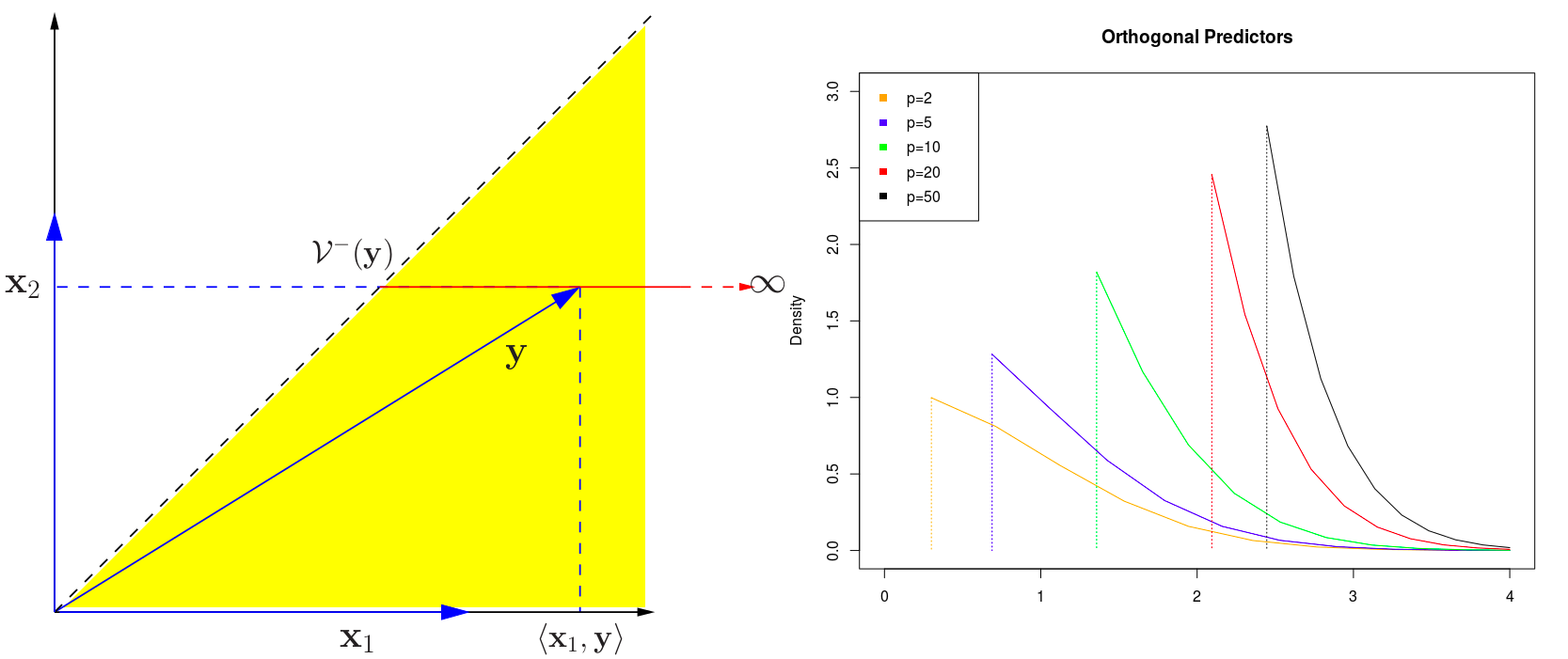
\[\begin{equation}\label{eq:uf} F_{\bfeta^T\bmu,\sigma^2\Vert\bfeta\Vert_2^2}^{\cV^-,\cV^+}(\bfeta^T\y)\mid\{\A\y\le b\}\sim U(0,1)\,. \end{equation}\]We can use this result to make conditional inferences about any linear functional $\bfeta^T\bmu$. For example, we can compute a p-value for testing $\bfeta^T\bmu = 0$. Not sure how to.
Or it just used this form to indicate that $\eta^T\y$ follows the distribution $F$
We can also construct a $1-\alpha$ level selection interval for $\theta=\bfeta^T\bmu$ by inverting this test, as follows. Let
\[P(\theta) = F_{\theta,\sigma^2\Vert\bfeta\Vert_2^2}^{\cV^-,\cV^+}(\bfeta^T\y)\mid\{\A\y\le b\}\,,\]the lower boundary of the interval is the largest value of $\theta$ such that $1-P(\theta) \le \alpha/2$, and the upper boundary is the smallest value of $\theta$ such that $P(\theta) \le \alpha/2$.
$P(\bfeta^T\y > x) = 1-F(x) = 1-P(\theta)$ and $P(\bfeta^T < x) = F(x) = P(\theta)$
I reproduced the orthogonal case of Example 6.1, where we consider the global null case, and found the predictor $j_1$ having largest absolute inner product with $\y$.
For the orthogonal case, $\cV^-$ is the second-largest among $\vert \x_k^T\y\vert$, while $\cV^+=\infty$.
library(mvtnorm)
set.seed(1234)
N = 60
genXY <- function(p, beta = matrix(0, p), rho = 0.5) {
    Sigma = matrix(rho, p, p)
    diag(Sigma) = rep(1, p)
    X = rmvnorm(N, rep(0, p), Sigma)
    X = apply(X, 2, function(x) {xc = x - mean(x); xc / sqrt(sum(xc^2))} )
    Y = X %*% beta + rnorm(N)
    return(list(X=X,Y=Y))
}
x = vector("list", 5)
fx = vector("list", 5)
p = c(2, 5, 10, 20, 50)
for (i in 1:5)
{
    for (j in 1:100)
    data = genXY(p[i], rho = 0)
    X = data$X
    Y = data$Y
    inner.products = apply(X, 2, function(x) { sum(x*Y) })
    j1 = which.max(abs(inner.products))
    V.minus = max(abs(inner.products[-j1]))
    x[[i]] = seq(V.minus, 4, length.out = 10)
    #px = (pnorm(x) - pnorm(V.minus)) / (1 - pnorm(V.minus))
    fx[[i]] = dnorm(x[[i]]) / (1 - pnorm(V.minus))
}
#plot(x, fx, type = "o")
plot(x[[1]], fx[[1]], type = "l", xlim = c(0, 4), ylim = c(0, 3), ylab = "Density", xlab = "", col = "orange", main = "Orthogonal Predictors")
segments(x[[1]][1], fx[[1]][1], x[[1]][1], 0, lty = 3, col = "orange")
lines(x[[2]], fx[[2]], col = "blue")
segments(x[[2]][1], fx[[2]][1], x[[2]][1], 0, lty = 3, col = "blue")
lines(x[[3]], fx[[3]], col = "green")
segments(x[[3]][1], fx[[3]][1], x[[3]][1], 0, lty = 3, col = "green")
lines(x[[4]], fx[[4]], col = "red")
segments(x[[4]][1], fx[[4]][1], x[[4]][1], 0, lty = 3, col = "red")
lines(x[[5]], fx[[5]], col = "black")
segments(x[[5]][1], fx[[5]][1], x[[5]][1], 0, lty = 3, col = "black")
legend("topleft",c("p=2","p=5", "p=10", "p=20", "p=50"),
       col = c("orange", "blue", "green", "red", "black"),
       pch = 15)
Fixed-$\lambda$ Inference for the Lasso
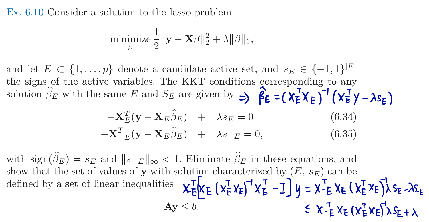
Consider the solution to the lasso, Apply \eqref{eq:uf} by constructing $\A$ and $b$ so that the event $\{\A\y\le b\}$ represents the set of outcome vectors $\y$ that yield the observed active set and signs of the predictors selected by the lasso at $\lambda$.
These inequalities derive from the subgradient conditions that characterize the solution,
This yields an active set $\cA$ of variables, and we can now make conditional inference on the population regression coefficients of $\y$ on $\X_\cA$. This means that we will perform a separate conditional analysis for $\bfeta$ equal to each of the columns of $\X_\cA(\X_{\cA}^T\X_{\cA})^{-1}$. Hence we can obtain exact p-values and confidence intervals for the parameter of the active set in the lasso solution at $\lambda$.
The Spacing Test for LAR
Apply \eqref{eq:uf} to successive steps of the LAR algorithm.
In the first step for testing the global null hypothesis, where $\bfeta_1^T\y=\lambda_1=\max_j\vert \langle \x_j,\y\rangle\vert$, and $\cV^-=\lambda_2,\cV^+=+\infty$, and hence the resulting test can be written in a very simple form:
\[R_1 = 1 - F_{0,\sigma^2}^{\cV^-,\cV^+}(\lambda_1\mid\{\A\y\le \b\}) = \frac{1-\Phi(\lambda_1/\sigma)}{1-\Phi(\lambda_2/\sigma)}\sim U(0,1)\,,\]which is known as spacing test for the global null hypothesis. Similarly, the tests are based on successive values for $\lambda_k$ would result in more complex expressions.
Comparison: the spacing test applies to each step of the sequential LAR procedure, and uses specific $\lambda$ values (the knots). In contrast, the fixed-$\lambda$ inference can be applied at any value of $\lambda$, but then treats this value as fixed.