Generalized Gradient Descent

Posted on Mar 20, 2019 (Update: Apr 08, 2019)

I read the topic in kiytay’s blog: Proximal operators and generalized gradient descent, and then read its reference, Hastie et al. (2015), and write some program to get a better understanding.

Projected Gradient

Suppose we want to minimize a convex differentiable function $f:\bbR^p\rightarrow \bbR$, a common first-order iterative method is gradient descent,

which has the alternative representation

Naturally, for minimization subject to a constraint $\beta\in\cC$:

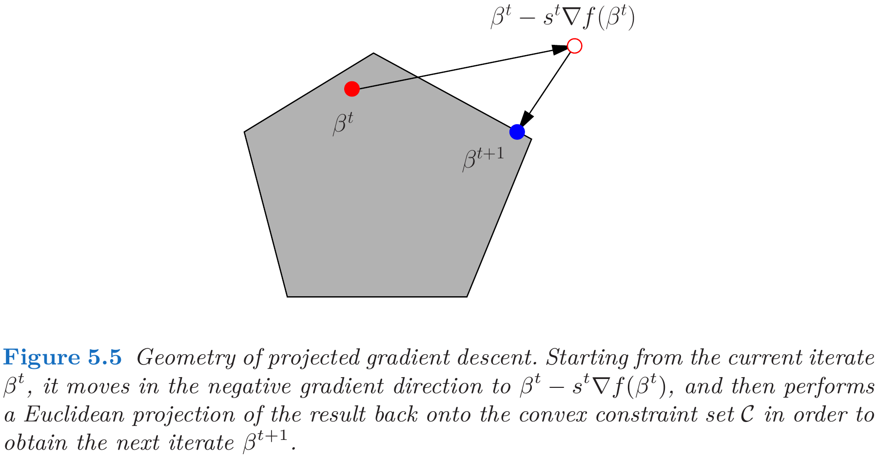
Proximal operator

Many objective functions $f$ can be decomposed as a sum $f=g+h$, where $g$ is convex and differentiable, and $h$ is convex but nondifferentiable. The generalized gradient descent update is defined by

Define the proximal map of a convex function $h$, a type of generalized projection operator:

More generally as mentioned in Boyd, S. (2010), define

as the proximity operator of $f$ with penalty $\rho$. And in variational analysis,

is called the Moreau envelope or Moreau-Yosida regularization of $f$.

Three examples can help us better understand it,

1. $h(z)=0$ for all $z\in\bbR^p$: $\prox_h(z)=z$
2. $h(z)=0$ if $z\in\cC$, and $h(z)=\infty$ otherwise: $\prox_h(z)=\argmin_{\beta\in\cC}{\Vert z-\beta\Vert^2_2}$.
3. $h(z)=\lambda\Vert z\Vert_1$ for some $\lambda\ge 0$: $\prox_h(z)=\cS_\lambda(z):=\sign(z)(\vert z\vert -\lambda)_+$.

With the notation of proximal operator,

Accelerated Gradient Methods

Nesterov (2007) proposed the class of accelerated gradient methods that use weighted combinations of the current and previous gradient directions.

Specifically, the accelerated gradient descent method involves a pair if sequence $\{\beta^t\}_{t=0}^\infty$ and $\{\theta^t\}_{t=0}^\infty$, and some initialization $\beta^0=\theta^0$. For iterations $t=0,1,\ldots,$ the pair is then updated according to the recursions

For non-smooth functions $f$ that have the “smooth plus non-smooth” decomposition $g+h$, Nesterov’s acceleration scheme can be combined with the proximal gradient update, that is, replace the above first step with the update

Example: Lasso

Take the lasso for example,

so that the proximal gradient update takes the form

which incorporates Nesterov’s acceleration.

Try to use the following Julia program to reproduce the simulation of Fig. 5.7 (Hastie et al. 2015),

using LinearAlgebra
using Distributions
using Random
Random.seed!(1234)
N = 1000
p = 500
ρ = 0.5
Σ = ones(p, p) * 0.5
Σ[diagind(Σ)] .= 1

X = rand(MvNormal(Σ), N)'

β = zeros(p)
β_idx = sample(1:p, 20, replace = false)
β[β_idx] .= randn(20)

Y = X * β + randn(N)
X_cov = 1/N * X' * X
st = 1 / eigen(X_cov).values[1]
function Sλ(θt, λ; st = st)
    z = θt + st * X' * (Y - X*θt) / N
    res = zeros(p)
    for i = 1:p
        if z[i] > st * λ
            res[i] = z[i] - st * λ
        elseif z[i] < - st * λ
            res[i] = z[i] + st * λ
        else
            res[i] = 0
        end
    end
    return res
end

function f(β, λ)
    return sum((Y - X * β).^2) / N * 0.5 + λ * sum(abs.(β))
end

function prox(T = 100; θ0 = zeros(p), λ = 0.7, Nesterov = true)
    β = zeros(p, T)
    θ = zeros(p, T)
    β[:,1] = Sλ(θ0, λ)
    θ[:,1] = β[:,1] + (β[:,1] - θ0) * 0 / (0 + 3) # θ1 = β1
    err = zeros(T)
    err[1] = f(β[:,1], λ)
    for t = 1:(T-1)
        β[:,t+1] = Sλ(θ[:,t], λ)
        if Nesterov
            θ[:,t+1] = β[:,t+1] + (β[:,t+1] - β[:,t]) * t / (t + 3)
        else
            θ[:,t+1] = β[:,t+1]
        end
        err[t+1] = f(β[:,t+1], λ)
    end
    return err, sum(β[:,T] .!= 0)
end

# run
res11, n11 = prox() # 5
res12, n12 = prox(Nesterov=false) # 102
# estimate beta_star with the last one (or the minimum one)
res1_min = minimum(vcat(res11, res12))
err11 = ( res11 .- res1_min ) / res1_min
err12 = ( res12 .- res1_min ) / res1_min

res21, n21 = prox(λ = 0.05) # 113
res22, n22 = prox(λ = 0.05, Nesterov = false) # 310
res2_min = minimum(vcat(res21, res22))
err21 = (res21 .- res2_min ) / res2_min
err22 = (res22 .- res2_min ) / res2_min

using Plots
p1 = plot(res11, label = "Proximal gradient",
            xlabel = "Number of Steps",
            ylabel = "Relative Error", title = "Sparse (lambda = 0.7)")
plot!(p1, res12, label = "Nesterov momentum")

p2 = plot(res21, label = "Proximal gradient",
            xlabel = "Number of Steps",
            ylabel = "Relative Error", title = "Dense (lambda = 0.05)")
plot!(p2, res22, label = "Nesterov momentum")

p = plot(p1, p2, layout = (1, 2), size = (1080, 720))
savefig(p, "res.png")

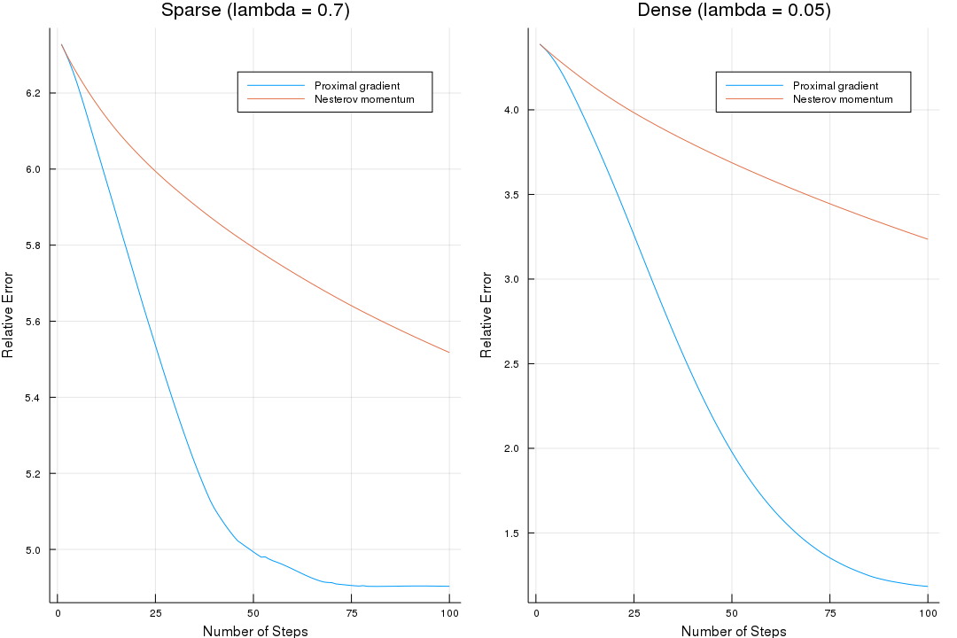
the tendency is almost completely same, but there are also some remarks I want to mentioned.

• $\beta^*$ is not necessarily the true $\beta$, because the object function also includes the penalty term.
• based on the previous fact, we need to estimate the true $\beta^*$, so I choose the minimum one (also should be the last one) during the iterations as the estimate.
• in my simulation, if $\lambda=0.7$, the number of nonzero entries in $\beta^*$ is only 5, while the original reports 20, similar result for $\lambda=0.05$, 113 v.s. 237.
• my relative error is also larger than the origin figure, which might related to the initial $\beta^0$, and the detailed simulation settings.

References

• kiytay’s blog: Proximal operators and generalized gradient descent
• Hastie, T., Tibshirani, R., & Wainwright, M. (2015). Statistical Learning with Sparsity. 362.
• Gradient methods for minimizing composite objective function, Technical Report 76, Center for Operations Research and Econometrics (CORE), Catholic University of Louvain (UCL).