Distributed inference for quantile regression processes

Posted on Mar 13, 2019

Tags: Quantile Regression, Divide-and-Conquer

This note is for Volgushev, S., Chao, S.-K., & Cheng, G. (2019). Distributed inference for quantile regression processes. The Annals of Statistics, 47(3), 1634–1662.

Abstract

the increased availability of massive data sets provides a unique opportunity to discover subtle patterns in their distributions,

propose a two-step procedure:

1. estimate conditional quantile functions at different levels in a parallel computing environment.
2. construct a conditional quantile regression process through projection based on these estimated quantile curves.

Introduction

1. Pioneering contributions on theoretical analysis of divide and conquer algorithms focus on mean squared error rates.
2. In the last two years, such procedures have been developed for various non- and semi-parametric estimation approaches that focus on the mean or other notions of central tendency.

Limitations:

1. Focus on the mean tendency illuminates one important aspect of the dependence between predictors and response, but ignores all other aspects of the dependence between predictors and response.
2. most of the work assumes homoskedastic (方差齐性) or sub-Gaussian tails.

Proposal

use quantile regression in order to extract features of the conditional distribution of the response while avoiding tail conditions and taking heteroskedasticity into account.

focus on estimating the conditional quantile function $x\mapsto Q(x;\tau):=F_{Y\mid X}^{-1}(\tau\mid x)$.

A flexible class of models for conditional quantile functions can be obtained by basis expansions of the form

\[Q(x;\tau)\approx \Z(x)^T\bbeta(\tau)\,.\]

Given data $\{(X_i,Y_i)\}_{i=1}^N$,

\[\hat\bbeta_{or}(\tau):=\arg\min_{\b\in \bbR^m}\sum_{i}^N\rho_\tau\{Y_i-\b^T\Z(X_i)\}\,,\]

where $\rho_\tau(u):=\{\tau-1(u\le 0)\}u$.

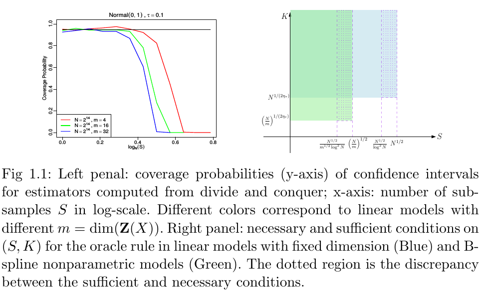
To utilize the divide and conquer approach where the full sample is randomly split across several computers into $S$ smaller sub-samples of size $n$, the minimization is solved on each sub-sample, and results are averaged in the end to obtain the final estimator $\bar\bbeta(\tau)$.

To obtain a picture of the entire conditional distribution of response given predictors, it requires to estimate the conditional quantile function at several quantile level.

Two step quantile projection algorithm:

1. use the divide and conquer to compute $\bar\bbeta(\tau_1),\ldots,\bar\bbeta(\tau_K)$ for a grid of quantile values $\tau_1,\ldots,\tau_K$.
2. compute a matrix $\hat \Xi$, which can be used to calculate the quantile projection estimator $\hat\bbeta(\tau)$. Based on $\hat\bbeta(\tau)$, we can estimate the conditional distribution function.

Conduct a detailed analysis of conditions to ensure the “oracle rule”:

• derive sufficient conditions for both $S$ and $K$, and necessary in some cases up to $\log N$ terms
• necessary and sufficient conditions on $K$.

The asymptotic distribution of $\hat\bbeta_{or}$ is typically not pivotal. Several ways to overcome this problem:

1. based on normal and t-approximations as well as a novel bootstrap procedure.
2. rely on estimating the asymptotic variance.