Approximate $\ell_0$-penalized piecewise-constant estimate of graphs
Posted on
Abstract
Object
Recovery of piecewise-constant signals on graphs by the estimator minimizing an $\ell_0$-edge-penalized objective.
Results
Although exact minimization of this objective may be computational intractable, the same statistical risk guarantees are achieved by the $\alpha$-expansion algorithm which computes an approximate minimizer in polynomial time.
- for graphs with small average vertex degree, these guarantees are minimax rate-optimal over classes of edge-sparse signals.
- for spatially inhomogeneous graphs, propose minimization of an edge-weighted objective where each edge is weighted by its effective resistance or another measure of its contribution to the graph’s connectivity. Establish minimax optimality of the resulting estimators over corresponding edge-weighted sparsity classes.
Theoretically these risk guarantees are not always achieved by the estimator minimizing the $\ell_1$/total-variation relaxation, and empirically that $\ell_0$-based estimates are more accurate in high signal-to-noise settings.
Introduction
Let $G=(V,E)$ be a known (undirected) graph. At each vertex $i$, an unknown value $\mu_{0,i}$ is observed with noise
\[Y_i = \mu_{0,i} + \varepsilon_i\,,\]where $\varepsilon_i\sim N(0,\sigma^2)$ independently and $G$ is (fully ?) connected.
A connected graph is any graph where there’s a path between every pair of vertices in the graph. A complete graph has an edge between every pair of vertices.
Goal
Estimating the true signal vector $\mu_0:=(\mu_{0,1},\ldots,\mu_{0,n})$ from observed data $Y:=(Y_1,\ldots,Y_n)$, where $\mu_0$ is (or is well approximated by) a piecewise-constant signal over $G$.
Applications
- Multiple change point detection:
- Image segmentation
- Anomaly identification in networks
Focus
The method of “$\ell_0$-edge-denoising”, which seeks to estimate $\mu_0$ by the values $\mu\in\bbR^n$ minimizing the residual squared error $\frac 12\Vert Y-\mu\Vert^2$ plus a penalty for each edge $\{i,j\}\in E$ where $\mu_i\neq\mu_j$. Formally, the objective function is
\[\qquad F_0(\mu):=\frac 12\Vert Y-\mu\Vert^2 + \lambda\Vert D\mu\Vert_0\,, \qquad \Vert D\mu\Vert_0=\1\{\mu_i\neq \mu_j\}\tag{L0}\label{L0}\]A more general weighted version of the above objective function
\[\qquad F_w(\mu):=\frac 12\Vert Y-\mu\Vert^2+\lambda \Vert D\mu\Vert_w\,,\qquad \Vert D\mu\Vert_w := \sum_{\{i,j\}\in E}w(i,j)\1\{\mu_i\neq\mu_j\}\tag{W}\label{W}\]The combinatorial nature of $\eqref{L0}$ and $\eqref{W}$ render exact minimization of these objectives computationally intractable for general graphs. A primary purpose of this paper is to show that approximate minimization is sufficient to obtain statistically rate-optimal guarantees.
Results summary
Polynomial-time algorithm
A polynomial-time algorithm using the $\alpha$-expansion procedure yields approximate minimizers $\hat\mu$ of $\eqref{L0}$ and $\eqref{W}$ that achieve the same statistical risk guarantees as the exact minimizers, up to constant factors.
Theoretical guarantees for $\ell_0$ denoising
For any graph $G$, the estimate $\hat\mu$ (exactly or approximately) minimizing $\eqref{L0}$ with $\lambda\asymp\sigma^2\log\vert E\vert$ satisfies an “edge-sparsity” oracle inequality
\[\bbE[\Vert \hat\mu-\mu_0\Vert^2] \lesssim \inf_{\mu\in \IR^n}\Vert \mu-\mu_0\Vert^2 + \sigma^2\max(\Vert D\mu\Vert_0,1)\log\vert E\vert\,.\]where $a\lesssim b$ if $a\le Cb$.
Comparison with $\ell_1$/total-variation denoising
An alternative to minimizing $\eqref{L0}$ is to minimize its $\ell_1$/total-variation relaxation,
\[\tag{TV} \label{TV}\qquad F_1(\mu):=\frac 12\Vert Y-\mu\Vert^2+\lambda\Vert D\mu\Vert_1\,,\qquad \Vert D\mu\Vert_1:=\sum_{\{i,j\}\in E}\vert \mu_i-\mu_j\vert\]One advantage of this approach is that $\eqref{TV}$ is convex and can be exactly minimized in polynomial time. However, whether the risk guarantees hold for $\hat\mu$ minimizing $\eqref{TV}$ depends on properties of the graph. In particular, they do not hold for the linear chain graph.
Edge-weighting for inhomogeneous graphs
When $G$ has regions of differing connectivity, $\Vert D\mu\Vert_0$ is not a spatially homogeneous measure of complexity, and it may be more appropriate to minimize the edge-weighted objective $\eqref{W}$ where $w(i,j)$ measures the contribution of edge $\{i,j\}$ to the connectivity of the graph. One such weighting weights each edge by its effective resistance when $G$ is viewed as an electrical resistor network.
Related Work
For change point problems where $G$ is the linear chain, $\eqref{L0}$ may be exactly minimized by dynamic programming in quadratic time. Pruning ideas may reduce runtime to be near-linear in practice. Correct change point recovery and distributional properties of $\hat\mu$ minimizing $\eqref{L0}$ were studied asymptotically when the number of true change points is fixed.
In image applications where $G$ is the 2D lattice, $\eqref{L0}$ is closely related to the Mumford-Shah functional and Ising/Potts-model energies for discrete Markov random fields. In the latter discrete setting, where each $\mu_i$ is allowed to take value in a finite set of “labels”, a variety of algorithms seek to minimize $\eqref{L0}$ using minimum s-t cuts on augmented graphs. For an Ising model with only two distinct labels, the exact minimizer may be computed via a single minimum s-t cut. For more than two distinct labels, exact minimization of $\eqref{L0}$ is NP-hard.
There is a large body of literature on the $l_1$-relaxation $\eqref{TV}$. This method and generalizations were suggested in different contexts and guises for the linear chain graph and also studied theoretically. A body of theoretical work establishes that $\hat\mu$ minimizing $\eqref{TV}$ is (or is nearly) minimax rate-optimal over signal classes of bounded variation for the linear chain graph and higher-dimensional lattices.
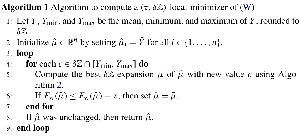
Approximation Algorithm
$\delta\bbZ$-expansion
For $\delta>0$, denote
\[\delta\bbZ:=\{...,-3\delta,-2\delta,-\delta,0,\delta,2\delta,3\delta,...\}\]as the set of all integer multiples of $\delta$. For any $\mu\in \bbR$, a $\delta\bbZ$-expansion of $\mu$ is any other vector $\tilde \mu\in \bbR^n$ such that there exists a single value $c\in \delta\bbZ$ for which, for every $i$, either $\tilde \mu_i=\mu_i$ or $\tilde \mu_i=c$. For $\delta>0$ and $\tau\ge 0$, a $(\tau,\delta\bbZ)$-local-minimizer of (W) is any $\mu\in\IR^n$ such that for every $\delta\bbZ$-expansion $\tilde \mu$ of $\mu$,
\[F_w(\mu)-\tau\le F_w(\tilde \mu)\,.\]Informally, a $\delta\bbZ$-expansion of $\mu$ can replace any subset of vertex values by a single new value $c\in\delta\bbZ$, and a $(\tau,\delta\bbZ)$-local-minimizer is such that no further $\delta\bbZ$-expansion reduces the objective value by more than $\tau$.
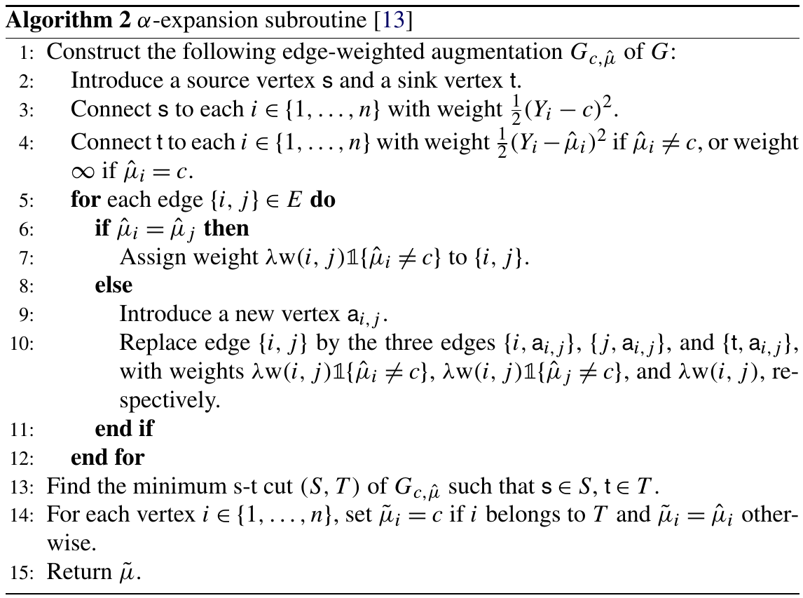
Minimum s-t cut
An s-t cut $C=(S,T)$ is a partition of $V$ such that $s\in S$ and $t\in T$. The cut-set $X_C$ of a cut $C$ is the set of edges that connect the source part of the cut to the sink part:
\[X_C:=\{(u,v)\in E:u\in S, v\in T\}=(S\times T)\cap E\]The capacity of an s-t cut is the total weight of its edges
\[c(S,T)=\sum_{(u,v)\in X_C}c_{uv}=\sum_{(i,j)\in E}c_{ij}d_{ij}\]The Minimum s-t cut problem is to maximize $c(S,T)$, that is, to determine $S$ and $T$ such that the capacity of the S-T cut is minimal.
Algorithms
Simulations
Study empirically the squared-errors of the approximate minimizers of $\eqref{L0}$ and $\eqref{W}$, as well as the minimizer of $\eqref{TV}$. Report the standardized mean-squared-error
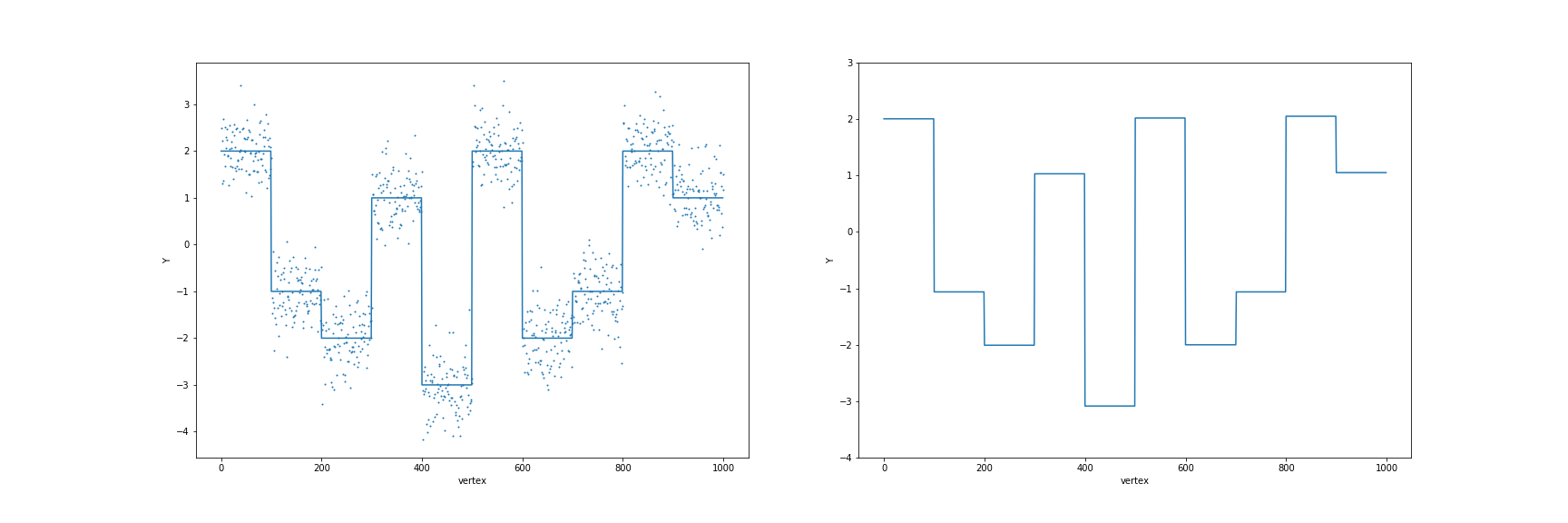
\[\frac{1}{n\sigma^2}\Vert \hat\mu-\mu_0\Vert^2\tag{st.MSE}\label{st.MSE}\]Linear chain graph
Use their software package, I wrote the following simple code to reproduce Fig. 1.
import numpy as np
n = 1000
mu = np.repeat([2, -1, -2, 1, -3, 2, -2, -1, 2, 1], 100)
data = mu + np.random.normal(size = n) * 0.5

from GraphSegment import Edges_1D, GraphSegment
edges = Edges_1D(n)
lamb = 0.5
res = GraphSegment(data, edges, lamb, delta=0.01)

import matplotlib.pyplot as plt
fig, (ax1, ax2) = plt.subplots(ncols = 2, figsize = (24, 8))
ax1.scatter(np.array(range(n))+1, data, s=1)
ax1.plot(mu)
ax1.set_xlabel("vertex")
ax1.set_ylabel("Y")

ax2.plot(res)
ax2.set_xlabel("vertex")
ax2.set_ylabel("Y")

plt.savefig("res.png")
The result is
Vary the noise levels $\sigma=0.1$ to $\sigma=1$, then calculate and compare the standard MSEs as follows:
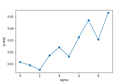
Note: It is important to choose penalty $\lambda$, the paper provides a method to choose the best $\lambda$, but here I take $\lambda=3$ by pilot studies for simplicity.