Gibbs Sampler for Finding Motif
Posted on (Update: )
This post is the online version of my report for the Project 2 of STAT 5050 taught by Prof. Wei.
Posterior distribution
Now we have a total of $N$ DNA sequences, $\R=(R_1,\ldots,R_N)$ with common length $L$. Let $\bftheta_0=(\theta_{01},\theta_{02},\theta_{03},\theta_{04})$ be the probability vector describing the residue frequencies outside a motif, or say these residues follow a common multinomial model with parameter $\bftheta_0$, where the number 1, 2, 3, 4 represent four types of nucleotide, A, G, C, T for simplicity. Let $\bftheta_j,j=1,\ldots,W$ represent the frequency of each base at the $j$-th position of the motif, and $\bfTheta = [\bftheta_1,\ldots,\bftheta_W]$. By treating the alignment data $A$ as missing data, we can write the complete-data likelihood of the parameters as
\[\begin{align*} \pi(\R, \A\mid \bftheta_0,\Theta) &\propto\bftheta_0^{\h(\R_{\{\A\}^c})}\prod_{j=1}^W\bftheta_j^{\h(\R_{\A(j)})}\,,%\\ %\propto \prod_{j=1}^W\Big(\frac{\bftheta_j}{\bftheta_0}\Big)^{\h(\R_{\A(j)})} \end{align*}\]where the notation is adopted from Liu et al. (1995). Specifically, ${\A}=\{(k, A_k+j-1):k=1,\ldots,N,j=1,\ldots,W\}$ represent the set of residue indices occupied by the motif elements with alignment variable $A$, in which $A_k$ is the starting position of the element of the $k$-th sequence. $\R_{{\A}} = \{r_{k,A_k+j-1}:k=1,\ldots,N;j=1,\ldots,W\}$ denote the collection of the residues, and $\A(j) = \{(k,A_k+j-1):k=1,\ldots,N\}$ is the set of the $j$-th positions of all elements. Also, $\h$ is the counting function, which counts how many of each type (A, G, C, T) in a DNA sequence. For general vectors $\v = (v_1,\ldots,v_p)^T$ and $\bftheta = (\theta_1,\ldots,\theta_p)^T$, we define $\bftheta^\v =\theta_1^{v_1}\cdots\theta_p^{v_p}$.
Collapsing $\bfTheta$
Let the prior of $\bftheta_0$, $f(\bftheta_0)$ be a Dirichlet distribution with parameter $\bfalpha = (\alpha_1,\ldots,\alpha_4)$, and let the prior of $\bfTheta$, $g(\bfTheta)$, be a product Dirichlet distribution with parameter $\bfbeta = (\bfbeta_1,\ldots,\bfbeta_W)$ and $\bfbeta_j=(\beta_{1j}, \ldots,\beta_{4j})^T$. Then by using the Bayes theorem and integrating out the $\bfTheta$,
\[\begin{align*} \pi(\A,\bftheta_0\mid\R) &\propto \pi(\R,\A,\bftheta_0)\\ &=\int \pi(\R,\A\mid\bftheta_0,\bfTheta)f(\bftheta_0)g(\bfTheta)d\bfTheta\\ &\propto \bftheta_0^{\h(\R_{\{\A\}^c})+\bfalpha -1}\prod_{j=1}^W\Gamma\{\h(\R_{\A(j)})+\bfbeta_j\}\,. \end{align*}\]Then we have \(\bftheta_0 \mid \A,\R \sim \mathrm{Dir}(\h(\R_{\{\A\}^c})+\bfalpha)\,.\)
Let $\A_{[-k]}$ denote the set ${(l,a_l),l\neq k}$, then
\[\begin{align} %\pi(A_k\mid \bftheta_0, \A_{[-k]},\R)\propto\frac{\Gamma\{\h(\R_{\{\A_{[-k]}\}^c})+\bfalpha-\h(\R_{A_k})\}}{\Gamma\{\h(\R_{\{\A_{[-k]}\}^c})+\bfalpha\}}\times \prod_{j=1}^W\{\h(\R_{\A_{[-k]}(j)})+\bfbeta_j\}^{\h(r_{k,A_k+j-1})}\,. \pi(A_k\mid \bftheta_0, \A_{[-k]},\R)&\propto\bftheta_0^{\h(\R_{\{\A\}^c})+\bfalpha -1}\times \prod_{j=1}^W\frac{\Gamma\{\h(\R_{\A(j)})+\bfbeta_j\}}{\Gamma\{\h(\R_{\A_{[-k]}(j)})+\bfbeta_j\}}\notag\\ &= \bftheta_0^{\h(\R_{\{\A_{[-k]}\}^c})-\h(\R_{\{A_k\}})+\bfalpha-1}\prod_{j=1}^W\{\h(\R_{\A_{[-k]}(j)})+\bfbeta_j\}^{\h(r_{k,A_k+j-1})}\notag\\ &\propto \bftheta_0^{-\h(\R_{\{A_k\}})}\prod_{j=1}^W\{\h(\R_{\A_{[-k]}(j)})+\bfbeta_j\}^{\h(r_{k,A_k+j-1})}\label{eq:mul}\,, \end{align}\]where the equality is due to
\[\begin{align*} \h(\R_{\{\A\}^c}) &= \h(\R_{\{\A_{[-k]}\}^c})-\h(\R_{\{A_k\}})\\ \h(\R_{\A(j)}) &= \h(\R_{\A_{[-k]}(j)}) + \h(r_{k,A_k+j-1}) \end{align*}\]and the fact that the components of $\h(r_{k,A_k+j-1})$ only take 0 or 1. Then
\[A_k\mid\bftheta_0,\A_{[-k]},\R\sim \mathrm{Multinomial}(p_{ki})\,,\]where
\[p_{ki} = \bftheta_0^{-\h(\R_{\{i\}})}\prod_{j=1}^W\{\h(\R_{\A_{[-k]}(j)})+\bfbeta_j\}^{\h(r_{k,i+j-1})}\]Shift Mode
Liu (1994) discussed the shift mode problem, which means that the Gibbs sampler will not enable a global change for all random components simultaneously. He proposed the following transition to encourage a global shifting.
For any integer $\delta$, let $\A+\delta = (A_1+\delta, \ldots,A_N+\delta)$. If one of the $A_k$ equals 1, we assume that $\A-1\equiv \A$; if one of the $A_k$ equals $L-W+1$, then $\A+1=\A$. These two cases can be treated as the termination of shifting. Suppose that the current state is $\A^{(k)}=\A$; first choose $\delta=+1$ or $-1$ with probability 1/2 each, and compute
\[p = \frac{\pi(\A+\delta)}{\pi(\A)}\]where
\[\pi(\A) \propto \prod_{j=1}^W n_{jA}(\R)!n_{jG}(\R)!n_{jC}(\R)!n_{jT}(\R)!\,,\]and $n_{jA}(\R)$ is the number of counts of nucleotide type $A$ among the $(A_k+j-1)$-th base of sequence $R_k$ for all $k=1,\ldots,N$, then update $\A^{(k+1)}=\A^{(k)}+\delta$ with probability $\min{p, 1}$, otherwise set $\A^{(k+1)}=\A^{(k)}$.
Gibbs sampler with Shifting
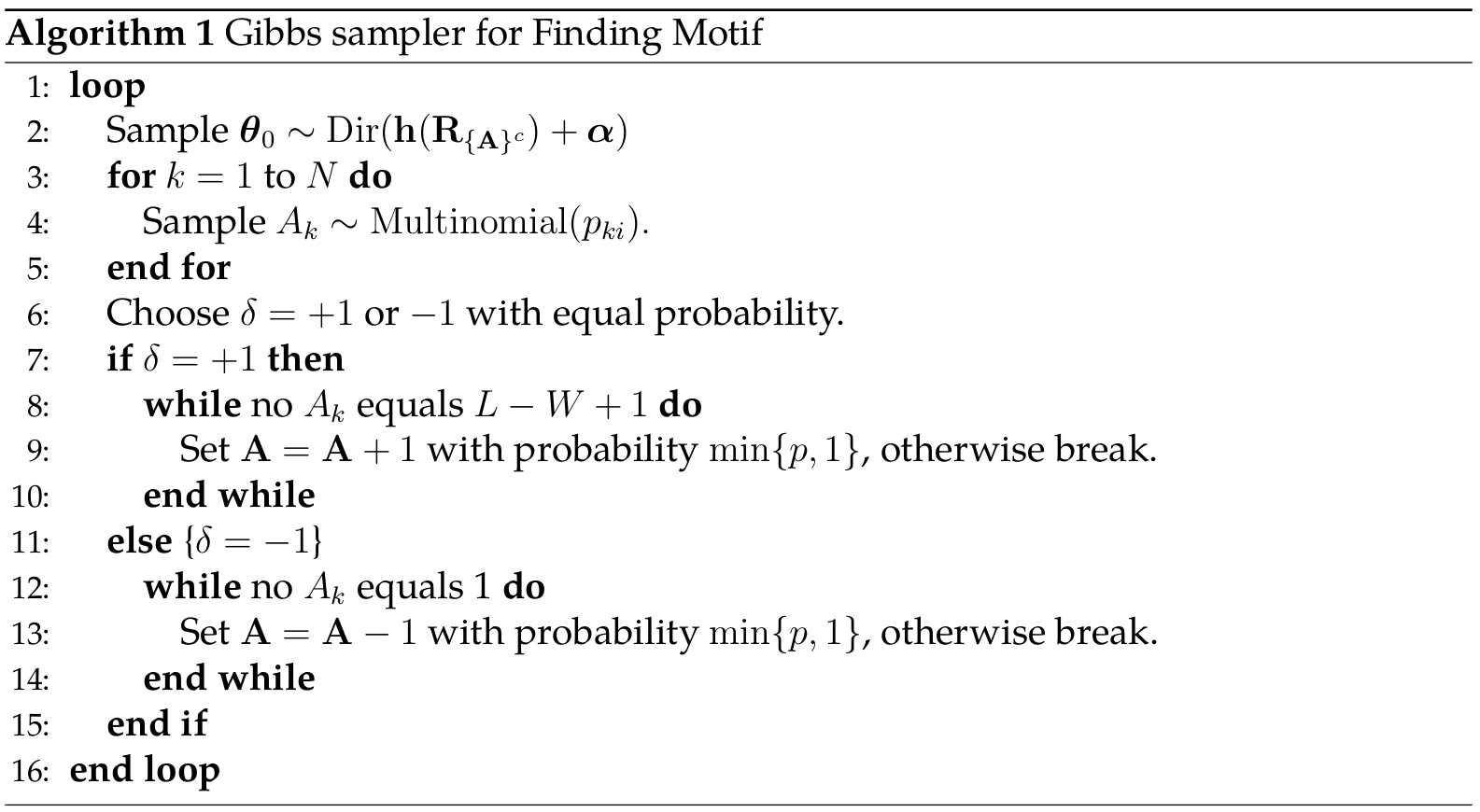
The implementation can be found in szcf-weiya/Gibbs-Motif.
Estimation
$\widehat \A$
Use the samples’ posterior mode $\widehat\A$ as the estimator of $\A$, and get the following sequence logo by submitting the result to http://weblogo.berkeley.edu/logo.cgi.
![]()
$\widehat\bftheta_0$
Use the sample’s posterior mean $\widehat\bftheta_0$ as the estimator of $\bftheta_0$, and we have \(\bftheta_0 = [0.208, 0.307, 0.314, 0.171].\)
$\widehat\bfTheta$
Base on the estimator $\widehat \A$, calculate the frequencies of each type of nucleotide on base $j, j=1,\ldots,W$, which can be the estimator of $\hat\bftheta_j$, and hence $\hat\bfTheta = [\hat\bftheta_1,\ldots,\hat\bftheta_W]$.
References
- Liu, J. S. (1994). The collapsed gibbs sampler in bayesian computations with applications to a gene regulation problem. Journal of the American Statistical Association, 89(427), 958–966.
- Liu, J. S., Neuwald, A. F., & Lawrence, C. E. (1995). Bayesian models for multiple local sequence alignment and gibbs sampling strategies. Journal of the American Statistical Association, 90(432), 1156–1170.