An R Package: Fit Repeated Linear Regressions
Posted on
Repeated Linear Regressions refer to a set of linear regressions in which there are several same variables.
Examples
Let’s start with the simplest situation, we want to fit a set of regressions which only differ in one variable. Specifically, denote the response variable as $y$, and these regressions are as follows.
\[\begin{array}{ll} y&\sim x_1 + cov_1 + cov_2+\ldots+cov_m\\ y&\sim x_2 + cov_1 +cov_2+\ldots+cov_m\\ \cdot &\sim \cdots\\ y&\sim x_n + cov_1 +cov_2+\ldots+cov_m\\ \end{array}\]where $cov_i, i=1,\ldots, m$ are the same variables among these regressions.
Similarly, the problem presented in the Background of the previous post is also Repeated Linear Regressions
Ideas
Intuitively, we can finish this task by using a simple loop in R code.
model = vector(mode='list', length=n)
for (i in 1:n)
{
  ...
  model[[i]] = lm(y~x)
}
However, it is not efficient in that situation. As we all know, in the linear regression, the main goal is to estimate the parameter $\beta$. And we have
\[\hat\beta = (X'X)^{-1}X'Y\]where $X$ is the design matrix and $Y$ is the observation of response variable.
It is obvious that there are some same elements in the design matrix, and the larger $m$ is, the more elements are the same. So I want to reduce the cost of computation by separating the same part in the design matrix.
Method
For the first example, the design matrix can be denoted as $X=(x, cov)$. If we consider intercept, it also can be seen as the same variable among these regression, so it can be included in $cov$ naturally. Then we have
\[(X'X)^{-1}= \left[ \begin{array}{cc} x'x & x'cov \\ cov'x & cov'cov \end{array} \right]= \left[ \begin{array}{ll} a& v'\\ v& B \end{array} \right]\]Woodbury formula:
\[(A+UCV)^{-1}=A^{-1}-A^{-1}U(C^{-1}+VA^{-1}U)^{-1}VA^{-1}\]
Let
\[A=\left[ \begin{array}{ll} a&O\\ O&B \end{array}\right],\; U=\left[ \begin{array}{ll} 1 & 0\\ O & v \end{array} \right],\; V= \left[ \begin{array}{ll} 0& v'\\ 1& O \end{array} \right]\]and $C=I_{2\times 2}$. Then we can apply woodbury formula,
\[(X'X)^{-1}=(A+UCV)^{-1}=A^{-1}-A^{-1}U(C^{-1}+VA^{-1}U)^{-1}VA^{-1}\]where
\[A^{-1}=\left[ \begin{array}{cc} a^{-1}&O\\ O&B^{-1} \end{array} \right]\]We can do further calculations to simplify and obtain the following result
\[(X'X)^{-1}=\left[ \begin{array}{cc} 1/a+\frac{a}{a-v'B^{-1}v}v'B^{-1}v & -\frac{v'B^{-1}}{a-v'B^{-1}v}\\ -\frac{B^{-1}v}{a-v'B^{-1}v} & B^{-1}+\frac{-B^{-1}vv'B^{-1}}{a-v'B^{-1}v} \end{array} \right]\]Notice that matrix $B$ is the same for all regression, the identical terms for each regression are just $a$ and $v$, which are very easy to calculate. So theoretically, we can reduce the cost of computation significantly.
For the second example, the previous post has discussed its details, so I just skip this part.
Package
You can install this package by
devtools::install_github('szcf-weiya/fRLR')
Let me check the results by two examples.
## use fRLR package
library(fRLR)
set.seed(123)
X = matrix(rnorm(50), 10, 5)
Y = rnorm(10)
COV = matrix(rnorm(40), 10, 4)
frlr1(X, Y, COV)

## use simple loop
res = matrix(nrow = 0, ncol = 2)
for (i in 1:ncol(X))
{
  mat = cbind(X[,i], COV)
  df = as.data.frame(mat)
  model = lm(Y~., data = df)
  tmp = c(i, summary(model)$coefficients[2, 4])
  res = rbind(res, tmp)
}
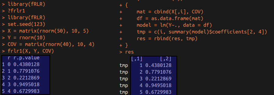
We can get the following results.

As we can see in the above figure, these p-values for the identical variable in each regression are equal betwwen two methods.
Similarly, we can test the second example
library(fRLR)
set.seed(123)
X = matrix(rnorm(50), 10, 5)
Y = rnorm(10)
COV = matrix(rnorm(40), 10, 4)

idx1 = c(1, 2, 3, 4, 1, 1, 1, 2, 2, 3)
idx2 = c(2, 3, 4, 5, 3, 4, 5, 4, 5, 5)

frlr2(X, idx1, idx2, Y, COV)

res = matrix(nrow=0, ncol=4)
for (i in 1:length(idx1))
{
  mat = cbind(X[, idx1[i]], X[,idx2[i]], COV)
  df = as.data.frame(mat)
  model = lm(Y~., data = df)
  tmp = c(idx1[i], idx2[i], summary(model)$coefficients[2,4], summary(model)$coefficients[3,4])
  res = rbind(res, tmp)
}
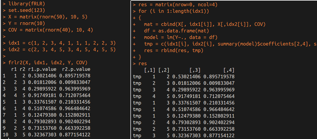
Again, we obtain the same results by different methods.

Computation Cost
The main aim of this new method is to reduce the computation cost. Now let’s compare its speed with the simple-loop method.
We can obtain the following time cost for $499\times 500/2=124750$ linear regressions.

It is obvious that the frlr method is much faster than the simple loop. Of course, there are many factors influence the speed, and the cost of the loop in R is very huge, while I realize the loop in Rcpp. So comparing two programs which both are in Rcpp might be much fairer. Actually, I have tested the similar results in the previous post in which the two programs are both in C++, only differ in their algorithm. As a result, separating the matrix in repeated linear regressions indeed can speed up the program.