An Illustration of Importance Sampling
Posted on (Update: )
This report shows how to use importance sampling to estimate the expectation.
We want to evaluate the quantity
\[\theta = \int_{\cal X}h(x)\pi(x)dx = E_{\pi}[h(x)]\]where $\pi(x)$ is pdf and $h(x)$ is the target function.
An Example
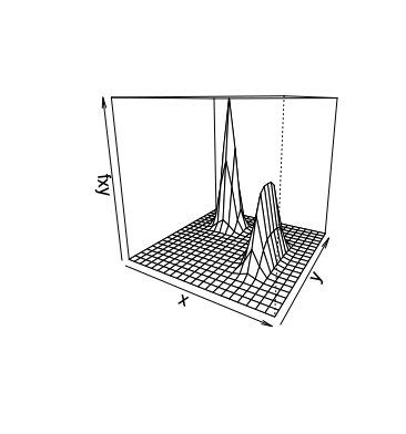
Consider a target function given by
\[f(x,y)=0.5\exp(-90(x-0.5)^2-45(y+0.1)^4)+\exp(-45(x+0.4)^2-60(y-0.5)^2)\]where $(x, y)\in [-1, 1]\times [-1,1]$.
We can plot the following function image

For mean, we have
\[\mu = E[f(x,y)] = \int f(x, y)\pi (x, y)dxdy = 4\int f(x,y)dxdy\]By taking $m$ random samplers, $(x^{(1)}, y^{(1)}), (x^{(2)}, y^{(2)}), \ldots, (x^{(m)}, y^{(m)})$, uniformly in $[-1,1]\times [-1, 1]$
then
\[\hat \mu = \frac{4}{m}\sum \limits_{i=1}^m f(x^{(i)}, y^{(i)})\]The implement code is as follows
Basic Idea
Suppose one is interested in evaluating
\[\mu = E_{\pi}(h(\mathbf x))=\int h(\mathbf x)\pi (\mathbf x)d\mathbf x\]The procedure of a simple form of the importance sampling algorithm is as follows.
- Draw $\mathbf x^{(1)}, \ldots, \mathbf x^{(m)}$ from a trial distribution $g$
- Calculate the importance weight $w^{(j)} = \pi (\mathbf x^{(j)})/ g(\mathbf x^{(j)}), \; for \; j=1, \ldots, m$
- Approximate $\mu$ by $\hat \mu = \frac{\sum_{j=1}^m w^{(j)}h(\mathbf x^{(j)})}{\sum_{j=1}^m w^{(j)}}$
The implementation code is as follows.