SIR and Its Implementation
Posted on (Update: ) 0 Comments
General Regression Model
\begin{equation} y=g(a+\mathbf x’\beta, \varepsilon)\,,\qquad \varepsilon\mid\mathbf x\sim F(\varepsilon)\,, \label{eq:model} \end{equation}
where the bivariate function $g$ is the link function, $F$ is the error distribution.
When the link function is arbitrary and unknown, we cannot estimate the entire parameter vector $(\alpha,\beta’)$. The most that can be identified for $(\alpha,\beta’)$ is the direction of the slope vector $\beta$, that is, the collection of the ratios $\{\beta_j/\beta_k,j,k=1,\ldots,d\}$. In other words, we can only determine the line generated by $\beta$, but not the length or the orientation of $\beta$.
Here, \eqref{eq:model} only involved a single $\beta$, for $k$ such unknown projection vector $\beta$, refer to Link-free v.s. Semiparametric
In some situations, the direction of $\beta$ might be the estimand of interest. For inference purposes, being able to identify the direction of $\beta$ means we can distinguish between $H_0:\beta_j=0$ and $H_A:\beta_j\neq 0$, that is, we can determine whether a specific regressor variable, say $x_j$, has an effect on the outcome. We can imagine the two dimensional case for illustration.
- Forward regression function
- Inverse regression function
\begin{equation} \xi(y)=\E(\x\mid y) \label{eq:irf} \end{equation}
Theorem
Assume the general regression model $\eqref{eq:model}$ and the design condition,
Design Condition: The regressor variable $\x$ is sampled randomly from a non-degenerate elliptically symmetric distribution.
The inverse regression function $\eqref{eq:irf}$ falls along a line:
\[\xi(y) = \mu + \Sigma\beta\kappa(y)\,,\]where $\mu=\E(\x),\Sigma=\cov(\x)$ and $\kappa(y)$ is a scalar function of $y$:
\[\kappa(y) = \frac{\E[(\x - \mu)'\beta\mid y]}{\beta'\Sigma\beta}\,.\]Corollary
Assume the same conditions in the above theorem. Let $\Gamma = \cov(\xi(y))$. The slope vector $\beta$ solves the following maximization problem:
\begin{equation} \max_{\b\in\IR^d}L(\b),\qquad\text{where}\; L(\b) = \frac{\b’\Gamma\b}{\b’\Sigma \b}\,. \label{eq:max} \end{equation}
The solution is unique (up to a multiplicative scalar) iff $\kappa(y)\not\equiv 0$.
Slicing (Inverse) Regression
Slicing (Inverse) Regression is a link-free regression method for estimating the direction of $\beta$. The method is based on a crucial relationship between the inverse regression $\E(\mathbf x\mid y)$ and the forward regression slope $\beta$.
Algorithm
- Estimate the inverse regression curve $\E(\mathbf x\mid y)$ using a step function: partition the range of $y$ into slices and estimate $\E(\mathbf x\mid y)$ in each slice of $y$ by the sample average of the corresponding $\mathbf x$’s;
- Estimate the covariance matrix $\Gamma=\Cov[\E(\mathbf x\mid y)]$, using the estimated inverse regression curve.
- Take the spectral decomposition of the estimate $\hat\Gamma$ with respect to the sample covariance matrix for $\mathbf x$. The principal eigenvector is the slicing regression estimate for the direction of $\beta$.
Empirical Algorithm
Empirically, suppose we have a random sample $\{(y_i,\x_i’),i=1,\ldots,n\}$.
Step 1
Partition the range of $y$ into $H$ slices, $\{s_1,\ldots,s_H\}$. For each slice of $y$, we estimate $\xi(y)=\E(\x\mid y)$ by the sample average of the corresponding $\x’s$:
\[\hat\xi(y)=\hat\xi_h=\frac{\sum_1^n\x_i1_{ih}}{\sum_{1}^n1_{ih}} \quad\text{if }y\in s_h\,,\]where $1_{ih}$ is the indicator for the event $y_i\in s_h$.
Denote
\[\xi_h = \E(\hat\xi_h) = \mu + \Sigma\beta k_h\,,\]where
\[k_h=\E[\kappa(y)\mid y\in s_h] = \frac{\E[(\x - \mu)'\beta\mid y\in s_h]}{\beta'\Sigma\beta}\,.\]Step 2
Introduce the following notations:
\begin{equation}
\begin{split}
p_h &= P(y\in s_h)\
\p &= (p_1,\ldots, p_H)’\
\k &= (k_1,\ldots, k_H)’\
\xi &= [\xi_1, \ldots, \xi_H]\
\hat\xi &= [\hat \xi_1,\ldots,\hat\xi_H]
\end{split}
\,.
\end{equation}
Estimate $\Gamma$ by
\[\hat\Gamma = \hat\xi W\hat\xi'\,,\]where $W$ is an arbitrary symmetric non-negative definite $H$ by $H$ matrix, chosen a priori, which satisfies $W\1 =0$.
Consider a maximization problem similar to $\eqref{eq:max}$:
\begin{equation} \max_{\b\in\IR^d}\hat L(\b),\qquad\text{where}\; \hat L(\b) = \frac{\b’\hat\Gamma\b}{\b’\hat\Sigma \b}\,, \label{eq:max2} \end{equation}
where $\hat\Sigma$ is the sample covariance matrix for the observed $\x$’s.
The solution to $\eqref{eq:max2}$, $\hat\beta$, is called slicing regression estimate for the direction of $\beta$. The slicing regression estimate $\hat\beta$ is the principal eigenvector for $\hat\Gamma$ with respect to the inner product
\[[\b,\v] = \b'\hat\Sigma\v\,.\]The optimal weight matrix is the so-called proportional to size (pps) weight matrix,
\[W^{(\p)} = D(\p) - \p\p';\quad \p'\1 = 1;\quad r_h\ge 0,\quad h=1,\ldots,H;\]where $D(\p)$ denotes the diagonal matrix with elements from the $H$-dimensional column vector $\p$.
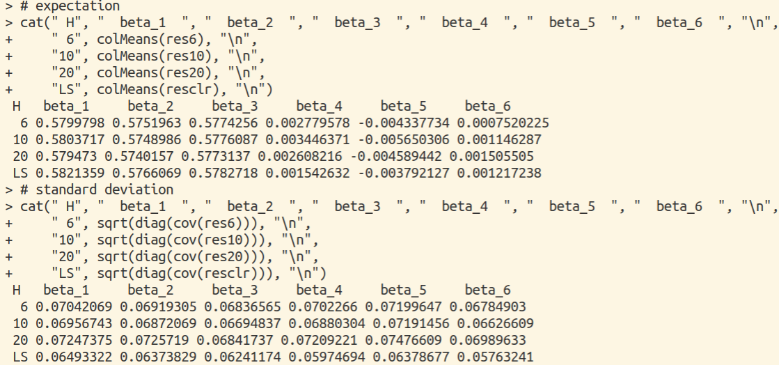
Simulation
Consider the following regression model
\[y=\x'\beta+\varepsilon\,,\]where $\beta=(1,1,1,0,0,0)’,\x\sim N(\0,I_6)$ and $\varepsilon\sim N(0,1)$. The main R program is as follows, and see simulation.R for complete source code.
sir <- function(x, y, H = 6)
{
    # slicing
    interval = seq(-3, 3, length = H-2 + 1)
    idx = vector("list", H)
    idx[[1]] = which( y <= -3 )
    idx[[H]] = which( y > 3)
    for (i in 1:(H-2))
    {
        idx[[i+1]] = which( y > interval[i] & y <= interval[i+1])
    }
    # calculate p
    p = sapply(idx, length) / length(y)
    # calculate `\hat \xi`
    xi = matrix(ncol = H, nrow = 6)
    for (i in 1:H)
    {
        if (length(idx[[i]]) == 0)
        {
            cat("ok\n")
            xi[, i] = rep(0, 6)
        }
        else if (length(idx[[i]]) == 1)
        {
            xi[, i] = x[ idx[[i]], ]
        }
        else
        {
            xi[, i] = colMeans(x[ idx[[i]], ])
        }
    }
    # construct weight matrix Wp
    W = diag(p) - p %*% t(p)
    # estimate `\hat \Gamma`
    Gamma = xi %*% W %*% t(xi)
    # sample variance
    Sigma = cov(x)
    # naive method
    # invsqrtSigma = solve(sqrtm(Sigma))
    ev = eigen(Sigma)
    invsqrtSigma = ev$vectors %*% diag( 1/sqrt(ev$values) ) %*% t(ev$vectors)
    mat = invsqrtSigma %*% Gamma %*% invsqrtSigma
    # the first principal
    alpha = eigen(mat) $ vectors
    b = invsqrtSigma %*% alpha[,1]
    if (b[1] < 0)
    {
        b = -b
    }
    return(b)
}
Here are something in the implementation I want to point out.
- Let $\balpha=\hat\Sigma^{1/2}\b$ when solving $\eqref{eq:max2}$, then it reduced to solve the first principal component of matrix $\Sigma^{-1/2}\hat\Gamma\Sigma^{-1/2}$.
- There might be some slices with no $\x_i$, so I directly set $\xi_i$ as $\0$ (not proper), but it doesn’t have much influence on the results.
We can reproduce the results in Fig. 7.1 of Duan and Li (1991):