Stochastic Epidemic Models
Posted on 0 Comments
Discuss three different methods for formulating stochastic epidemic models.
Three Different Methods
There are three different methods for formulating stochastic epidemic models that relate directly to their deterministic counterparts.
- DTMC(discrete time Markov chain): time discrete, and state variables discrete
- CTMC(continuous time Markov chain): time continuous, but state variables discrete
- SDE(stochastic differential equation): time continuous, and state variables continuous
SIS and SIR
There are three classifications in SIS and SIR epidemic models according to disease status, susceptible, infectious and immune, and denoted them as $S, I, R$ respectively.
SIS
Two additional assumptions are made to simplify.
- No vertical transmission of the disease (all individuals are born susceptible)
- No disease-related deaths.
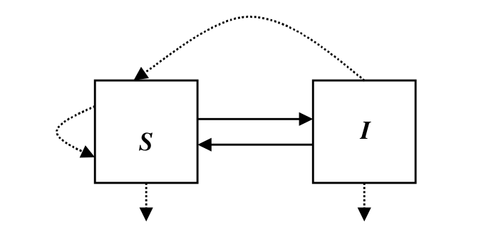
The following compartmental diagram illustrates the dynamic of the SIS epidemic model, where solid arrows denote infection or recovery, and dotted arrows denote birth or deaths.
We can use the differential equations to capture their relationship.
\[\begin{eqnarray} \frac{dS}{dt} &=& -\frac{\beta}{N}SI+(b+\gamma)I\\ \frac{dI}{dt} &=& \frac{\beta}{N}SI-(b+\gamma)I \end{eqnarray}\]where $\beta>0$ is the contact rate, $\gamma>0$ is the recovery rate, $b\ge 0$ is the birth rate, and $N=S(t)+I(t)$ is the total population size.
SIR
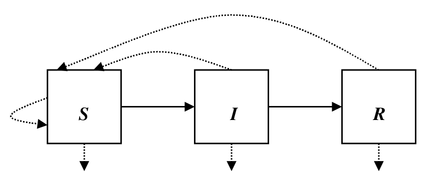
The following compartmental diagram illustrate the relationship between the three disease statuses, susceptible, infectious and immune.
Use differential equations to describe their relationship, we have
\[\begin{eqnarray} \frac{dS}{dt} &=& -\frac{\beta}{N}SI+b(I+R)\\ \frac{dI}{dt} &=& \frac{\beta}{N}SI-(b+\gamma)I\\ \frac{dR}{dt} &=& \gamma I-bR \end{eqnarray}\]where $\beta>0, \gamma>0, b\ge 0$, and the total population size satisfies $N=S(t)+I(t)+R(t)$。
Formulation of DTMC Epidemic Models
SIS
In an SIS epidemic model, there is only one independent random variable, $\cal I(t)$, because $\cal S(t)=N-I(t)$. The stochastic process ${\cal I(t)}_{t=0}^{\infty}$ has an associated probability function,
\[p_i(t)=Prob\{\cal I(t)=i\}\]for $i=0, 1,2,\ldots, N$ and $t=0, \Delta t, 2\Delta t,\ldots$, where
\[\sum\limits_{i=0}^Np_i(t)=1\]Denote $p(t)=(p_0(t), p_1(t), \ldots, p_N(t))^T$ as the probability vector associated with $\cal I(t)$. The stochastic process has the Markov property if
\[Prob\{\cal I(t+\Delta t)\mid I(0), I(\Delta t),\ldots, \cal I(t)\}=Prob\{\cal I(t+\Delta t)\mid \cal I(t)\}\]The probability of a transition from state $\cal I(t)=i$ to state $\cal I(t+\Delta t)=j,i\rightarrow j$, in time $\Delta t$, is denoted as
\[p_{ji}(t+\Delta t, t)=Prob\{\cal I(t+\Delta t)=j\mid \cal I(t)=i\}\]To reduce the number of transitions in time $\Delta t$, we make one more assumption. The time step $\Delta t$ is chose sufficiently small such that the number of infected individuals changes by at most one during the time interval $\Delta t$, that is,
\[i\rightarrow i+1, \; i\rightarrow i-1,\; or\; i\rightarrow i\]The transition probabilities for the DTMC epidemic model satisfy
\[p_{ji}(\Delta t)=\left\{ \begin{array}{ll} \frac{\beta i(N-i)}{N}\Delta t& j=i+1\\ (b+\gamma)i\Delta t&j=i-1\\ 1-[\frac{\beta i(N-i)}{N}+(b+\gamma)i]\Delta t & j=i\\ 0, & j\neq i+1, i, i-1 \end{array} \right.\]where the probability from state $i$ to state $i+1$ is the probability of a new infection, the probability from state $i$ to state $i-1$ is the probability of a death or recovery, and the probability from state $i$ to state $i$ is the probability of no change in states.
To simplify the notation, we have
\[p_{ji}(\Delta t)=\left\{ \begin{array}{ll} b(i)\Delta t& j=i+1\\ d(i)\Delta t&j=i-1\\ 1-[b(i)+d(i)]\Delta t & j=i\\ 0, & j\neq i+1, i, i-1 \end{array} \right.\]Then we can get the probabilities
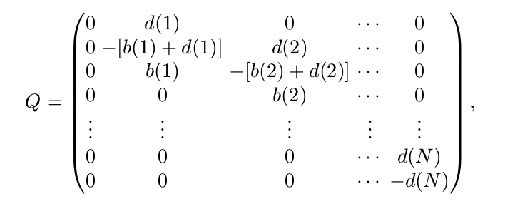
\[p_i(t+\Delta t)=p_{i-1}(t)b(i-1)\Delta t+p_{i+1}(t)d(i+1)\Delta t+p_i(t)(1-(b(i)+d(i))\Delta t)\]Finally, the transition matrix $P(\Delta t)$ is a $(N+1)\times (N+1)$ tridiagonal matrix given by
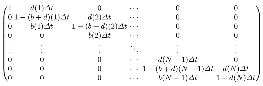
where $(b+d)(i)=b(i)+d(i)$.
It is worthy noting that the column sums, rather than row sums, equal one, so the transition equation would be
\[p(t+\Delta t)=P(\Delta t)p(t)\]SIR
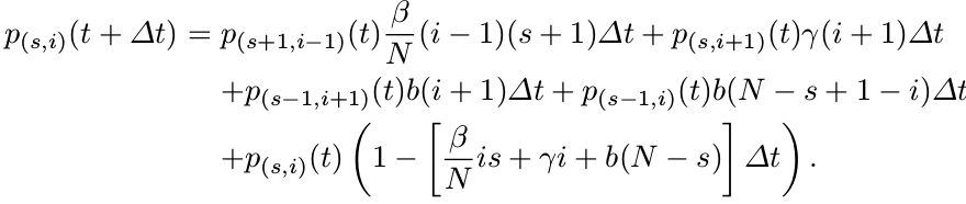
There are two independent random variables, $\cal S(t)$ and $\cal I(t)$. The random variable $\cal R(t)=N-S(t)-I(t)$. The bivariate process ${\cal S(t), \cal I(t)}_{t=0}^\infty$ has a joint probability function given by
\[p_{(s, i)}(t)=Prob\{\cal S(t)=s, \cal I(t)=i\}\]Transition probabilities can be defined based on the assumptions in the SIR deterministic formulation. First, assume that $\Delta t$ can be chosen sufficiently small such that at most one change in state occurs during the time interval $\Delta t$. The transition probabilities are denoted as follows:
\[p_{(s+k, i+j), (s,i)}(\Delta t)=Prob\{(\Delta \cal S, \Delta \cal I)=(k, j)\mid (\cal S(t), I(t))=(s, i)\}\]where $\Delta \cal S=S(t+\Delta t)-S(t)$. Hence,
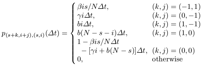
Then applying the Markov property, we can write the probability $p_{(s,i)}(t+\Delta t)$ as
Formulation of CTMC Epidemic Models
SIS
The stochastic process depends on the collection of discrete random variables ${\cal I(t)},t\in [0,\infty)$ and their associated probability functions $p(t)=(p_0(t), \ldots, p_N(t))^T$, where
\[p_i(t)=Prob\{\cal I(t)=i\}\]The stochastic process has the Markov property, that is
\[Prob\{\cal I(t_{n+1})\mid \cal I(t_0),I(t_1),\ldots,\cal I(t_n)\} = Prob\{\cal I(t_{n+1})\mid \cal I(t_n)\}\]for any sequence of real numbers satisfying $0\le t_0\le t_1\le \cdots \le t_n\le t_{n+1}$. And we have the infinitesimal transition probabilities are defined as follows:
\[p_{ji}(\Delta t)=\left\{ \begin{array}{ll} \frac{\beta i(N-i)}{N}\Delta t+o(\Delta t)& j=i+1\\ (b+\gamma)i\Delta t+o(\Delta t)&j=i-1\\ 1-[\frac{\beta i(N-i)}{N}+(b+\gamma)i]\Delta t+o(\Delta t) & j=i\\ o(\Delta t), & j\neq i+1, i, i-1 \end{array} \right.\]Similar to the SIS epidemic in DTMC, we have
\[p_i(t+\Delta t)=p_{i-1}(t)b(i-1)\Delta t+p_{i+1}(t)d(i+1)\Delta t+p_i(t)(1-(b(i)+d(i))\Delta t)+o(\Delta t)\]Subtracting $p_i(t)$, dividing by $\Delta t$, and letting $\Delta t\rightarrow 0$, leads to
\[\frac{dp_i}{dt}=p_{i-1}b(i-1)+p_{i+1}d(i+1)-p_i[b(i)+d(i)]\]for $i=1,2,\ldots, N$ and $dp_0/dt=p_1d(1)$. We can rewrite it by using matrix notation.
\[\frac{dp}{dt}=Qp\]where
It is worthy noting that the transition matrix $P(\Delta t)$ of the DTMC model and the matrix $Q$ called the infinitesimal generator matrix or generator matrix are related as follows:
\[Q=\lim_{\Delta t\rightarrow 0}\frac{P(\Delta t)-I}{\Delta t}\]SIR
Apply the derivation similar to the SIS epidemic to SIR epidemic model. For the sake of simplicity, I decide to skip this section. More details can be found in the reference listed at the end of this post.
Formulation of SDE Epidemic Model
Considering the much more difficult derivation of SDE and its merely little use for my current work, I skip the details about derivation. If you are interested in this part, you can refer to the bibliography at the end of this post.
References
Allen L. An introduction to stochastic epidemic models. Mathematical epidemiology. 2008:81-130.