A Bayesian Missing Data Problem
Posted on 0 Comments
Problem
There is an artificial dataset of bivariate Gaussian observation with missing parts. The symbol * indicates that the value is missing.
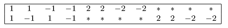
Denote these data as $y_1,\ldots, y_{12}$, where $y_t=(y_{t,1}, y_{t,2}), t=1,\ldots, 12$. The posterior distribution of $\rho$ given the incomplete data is of interest.
Firstly, the covariance matrix of the bivariate normal is assigned the Jeffrey’s noinformative prior distribution
\[\pi(\Sigma) \propto \vert \Sigma\vert^{-\frac{d+1}{2}}\]where $d$ is the dimensionality and equals to 2 in this problem. The posterior distribution of $\Sigma$ given $t$ i.i.d. observed complete data $y_1,\ldots, y_t$ is
\[p(\Sigma \mid y_1, \ldots, y_t) \propto \vert\Sigma \vert^{-\frac{d+1+t}{2}}exp\{-\frac{1}{2}tr[\Sigma^{-1} \cdot S]\}\]where $S = (s_{ij})_{22}, s_{ij}=\sum_{s=1}^t y_{s,i}y_{s,j}$.
By letting ${\cal Z}=\Sigma^{-1}$, then ${\cal Z}\sim Wishart(t, S)$.
For this problem,
\[p(\Sigma, \mathbf y_{mis}\mid \mathbf y_{obs}) \propto \vert\Sigma \vert^{-\frac{2+1+12}{2}}exp\{-\frac{1}{2}tr[\Sigma^{-1} \cdot S(\mathbf y_{mis})]\}\]where $S(\mathbf y_{mis})$ emphasizes that its value depends on the value of $\mathbf y_{mis}$. We can obtain the posterior distribution of $\Sigma$ by integrating out $\mathbf y_{mis}$. An importance sampling algorithm for achieving this goal can be implemented as follows:
- Sample $\Sigma$ from some trial distribution $g_0(\Sigma)$
- Draw $\mathbf y_{mis}$ from $p(\mathbf y_{mis}\mid \mathbf y_{obs},\Sigma)$
It is obvious that the predictive distribution of $\mathbf y_{mis}$ is simply the Gaussian distribution given $\Sigma$. So the key question is how to draw $\Sigma$. A simple idea is to draw $\Sigma$ from its posterior distribution conditional only on the first four complete observations:
\[g_0(\Sigma) \propto \vert \Sigma\vert^{-7/2}exp(-tr[\Sigma^{-1}S_4]/2)\]where $S_4$ is the sum of the square matrix computed from the first four observations.
Implement
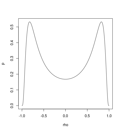
The analytical form is
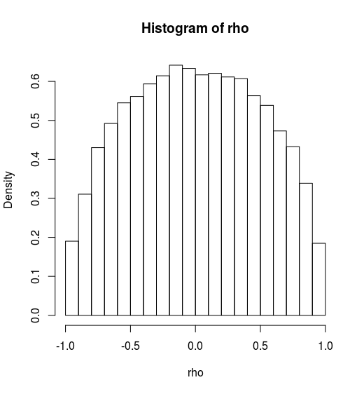
However, there might be some wrong in my code. You can find my code in Github.
Notes
If $X_1,\ldots, X_n; X_i\in R^p$ are $n$ independent multivariate Gaussians with mean $\mathbf 0$ and covariance matrix $\Sigma$, the distribution of $S = X’X\sim \cal W_p(\Sigma, n)$, and $S^{-1}\sim W_p^{-1}(\Sigma^{-1}, n)$, where $X = (X_1, X_2,\ldots, X_n)’$.
References
Liu, Jun S. Monte Carlo strategies in scientific computing. Springer Science & Business Media, 2008.